House Price Prediction – Data Normalization

Data Cleaning

1. Introduction

Data cleaning is a step in machine learning (ML) which involves identifying and removing any missing, duplicate or irrelevant data.

• Raw data (log file, transactions, audio /video recordings, etc) is often noisy, incomplete and inconsistent which can negatively impact the accuracy of model.
• The goal of data cleaning is to ensure that the data is accurate, consistent and free of errors.
• Clean datasets also important in EDA (Exploratory Data Analysis) which enhances the interpretability of data so that the right actions can be taken based on insights

2. What is Data Cleansing?

Data Cleansing is a data preprocessing step that focuses on:

• Detecting errors in raw data
• Fixing inconsistencies
• Removing unnecessary or harmful data

The goal is to produce a dataset that is:

• Accurate
• Consistent
• Reliable
• Suitable for analysis and machine learning models

Data cleansing is a critical part of Data Preparation and is performed before:

• Exploratory Data Analysis (EDA)
• Feature Engineering
• Data Normalization
• Model Training

3. How to Perform Data Cleaning

The process begins by identifying issues like missing values, duplicates and outliers. Performing data cleaning involves a systematic process to identify and remove errors in a dataset. The following steps are essential to perform data cleaning:

• Remove Unwanted Observations: Eliminate duplicates, irrelevant entries or redundant data that add noise.
• Fix Structural Errors: Standardize data formats and variable types for consistency.
• Manage Outliers: Detect and handle extreme values that can skew results, either by removal or transformation.
• Handle Missing Data: Address gaps using imputation, deletion or advanced techniques to maintain accuracy and integrity.

4. Implementation for Data Cleaning

Step 1: Import Libraries and Load Dataset

Import all the necessary libraries i.e pandas and numpy.

import pandas as pd
import numpy as np

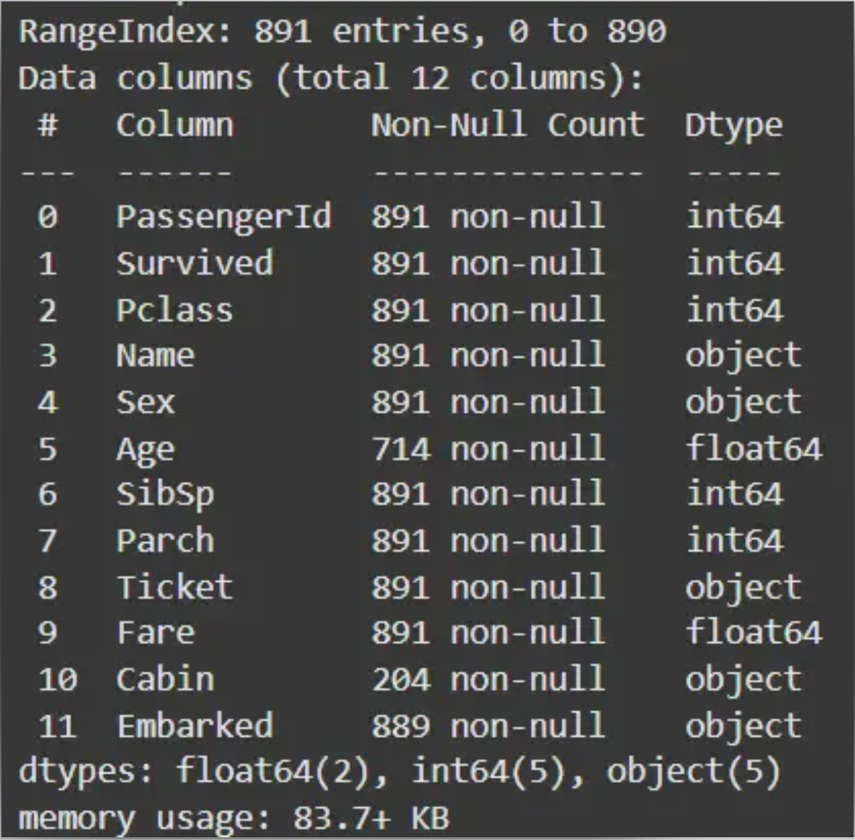
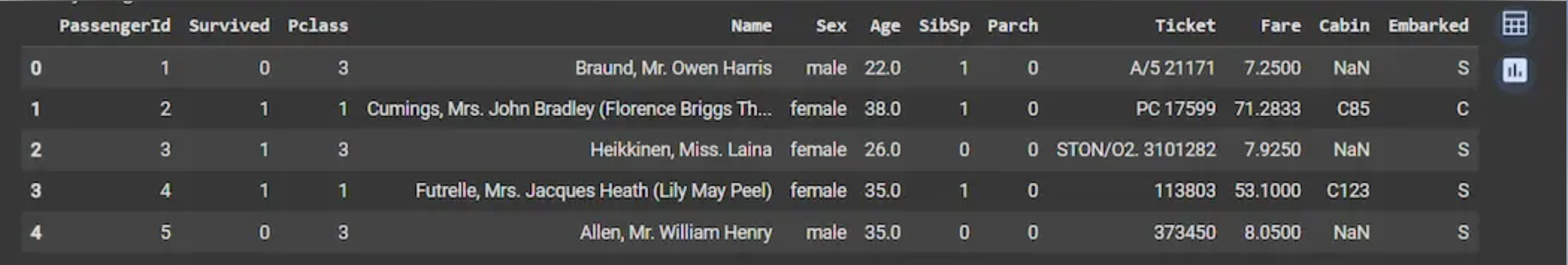
df = pd.read_csv('Titanic-Dataset.csv')
df.info()
df.head()

Output:

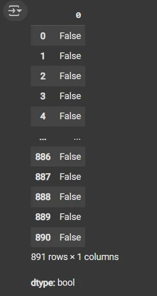
Step 2: Check for Duplicate Rows

df.duplicated(): Returns a boolean Series indicating duplicate rows.

df.duplicated()

Output:

Step 3: Identify Column Data Types

• List comprehension with .dtype attribute to separate categorical and numerical columns.
• object dtype: Generally used for text or categorical data.

cat_col = [col for col in df.columns if df[col].dtype == 'object']
num_col = [col for col in df.columns if df[col].dtype != 'object']

print('Categorical columns:', cat_col)
print('Numerical columns:', num_col)

Output:

Categorical columns: ['Name', 'Sex', 'Ticket', 'Cabin', 'Embarked']
Numerical columns: ['PassengerId', 'Survived', 'Pclass', 'Age', 'SibSp', 'Parch', 'Fare']

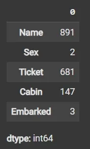
Step 4: Count Unique Values in the Categorical Columns

df[numeric_columns].nunique(): Returns count of unique values per column.

df[cat_col].nunique()

Output:

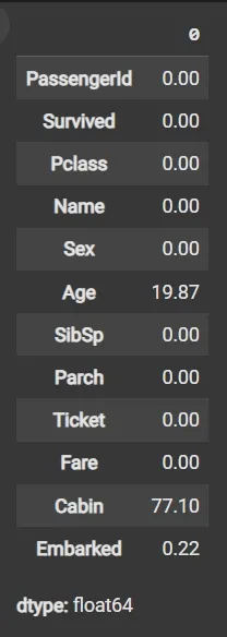
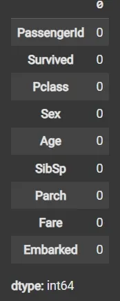
Step 5: Calculate Missing Values as Percentage

• df.isnull(): Detects missing values, returning boolean DataFrame.
• Sum missing across columns, normalize by total rows and multiply by 100.

round((df.isnull().sum() / df.shape[0]) * 100, 2)

Output:

Step 6: Drop Irrelevant or Data-Heavy Missing Columns

• df.drop(columns=[]): Drops specified columns from the DataFrame.
• df.dropna(subset=[]): Removes rows where specified columns have missing values.
• fillna(): Fills missing values with specified value (e.g., mean).

df1 = df.drop(columns=['Name', 'Ticket', 'Cabin'])
df1.dropna(subset=['Embarked'], inplace=True)
df1['Age'].fillna(df1['Age'].mean(), inplace=True)

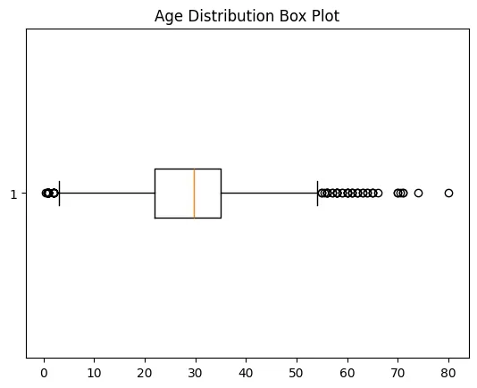
Step 7: Detect Outliers with Box Plot

• matplotlib.pyplot.boxplot(): Displays distribution of data, highlighting median, quartiles and outliers.
• plt.show(): Renders the plot.

import matplotlib.pyplot as plt

plt.boxplot(df3['Age'], vert=False)
plt.ylabel('Variable')
plt.xlabel('Age')
plt.title('Box Plot')
plt.show()

Output:

Step 8: Calculate Outlier Boundaries and Remove Them

• Calculate mean and standard deviation (std) using df[‘Age’].mean() and df[‘Age’].std().
• Define bounds as mean ± 2 * std for outlier detection.
• Filter DataFrame rows within bounds using Boolean indexing.

mean = df1['Age'].mean()
std = df1['Age'].std()

lower_bound = mean - 2 * std
upper_bound = mean + 2 * std

df2 = df1[(df1['Age'] >= lower_bound) & (df1['Age'] <= upper_bound)]

Step 9: Impute Missing Data Again if Any

• fillna() applied again on filtered data to handle any remaining missing values.

df3 = df2.fillna(df2['Age'].mean())
df3.isnull().sum()

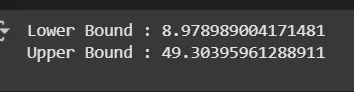
Step 10: Recalculate Outlier Bounds and Remove Outliers from the Updated Data

• mean = df3[‘Age’].mean(): Calculates the average (mean) value of the Age column in the DataFrame df3.
• std = df3[‘Age’].std(): Computes the standard deviation (spread or variability) of the Age column in df3.
• lower_bound = mean - 2 * std: Defines the lower limit for acceptable Age values, set as two standard deviations below the mean.
• upper_bound = mean + 2 * std: Defines the upper limit for acceptable Age values, set as two standard deviations above the mean.
• df4 = df3[(df3[‘Age’] >= lower_bound) & (df3[‘Age’] <= upper_bound)]: Creates a new DataFrame df4 by selecting only rows where the Age value falls between the lower and upper bounds, effectively removing outlier ages outside this range.

mean = df3['Age'].mean()
std = df3['Age'].std()

lower_bound = mean - 2 * std
upper_bound = mean + 2 * std

print('Lower Bound :', lower_bound)
print('Upper Bound :', upper_bound)

df4 = df3[(df3['Age'] >= lower_bound) & (df3['Age'] <= upper_bound)]

Output:

Step 11: Data validation and verification

Data validation and verification involve ensuring that the data is accurate and consistent by comparing it with external sources or expert knowledge. For the machine learning prediction we separate independent and target features. Here we will consider only ‘Sex’ ‘Age’ ‘SibSp’, ‘Parch’ ‘Fare’ ‘Embarked’ only as the independent features and Survived as target variables because PassengerId will not affect the survival rate.

X = df3[['Pclass','Sex','Age', 'SibSp','Parch','Fare','Embarked']]
Y = df3['Survived']

Step 12: Data formatting

Data formatting involves converting the data into a standard format or structure that can be easily processed by the algorithms or models used for analysis. Here we will discuss commonly used data formatting techniques i.e. Scaling and Normalization.

Scaling involves transforming the values of features to a specific range. It maintains the shape of the original distribution while changing the scale. It is useful when features have different scales and certain algorithms are sensitive to the magnitude of the features. Common scaling methods include:

1. Min-Max Scaling: Min-Max scaling rescales the values to a specified range, typically between 0 and 1. It preserves the original distribution and ensures that the minimum value maps to 0 and the maximum value maps to 1.

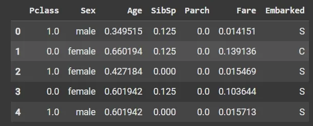
from sklearn.preprocessing import MinMaxScaler

scaler = MinMaxScaler(feature_range=(0, 1))

num_col_ = [col for col in X.columns if X[col].dtype != 'object']
x1 = X
x1[num_col_] = scaler.fit_transform(x1[num_col_])
x1.head()

Output:

Standardization (Z-score scaling): Standardization transforms the values to have a mean of 0 and a standard deviation of 1. It centers the data around the mean and scales it based on the standard deviation. Standardization makes the data more suitable for algorithms that assume a Gaussian distribution or require features to have zero mean and unit variance.

\[Z = (X - μ) / σ\]

Where:

• X = Data
• μ = Mean value of X
• σ = Standard deviation of X

Data Normalization

Data normalization is a preprocessing method that resizes the range of feature values to a specific scale, usually between 0 and 1. It is a feature scaling technique used to transform data into a standard range. Normalization ensures that features with different scales or units contribute equally to the model and improves the performance of many machine learning algorithms.

Key Features of Normalization:

• Maps the minimum and maximum of a feature to a defined range
• Preserves the relative relationships of the original data
• Useful for algorithms that rely on distance metrics such as k-Nearest Neighbours and clustering

Why do we need Normalization?

Machine learning models often assume that all features contribute equally. Features with different scales can dominate the model’s behavior if not scaled properly. Using normalization, we can:

• Ensure Equal Contribution of Features: Prevents features with larger scales from dominating models that are sensitive to magnitude such as K-Nearest Neighbours or neural networks. Improve Model Performance: Algorithms that rely on distances or similarities (KNN, K-Means clustering) perform better when features are normalized.
• Accelerate Convergence: Helps gradient-based algorithms like logistic regression or neural networks converge faster by keeping feature values in a similar range.
• Maintain Interpretability of Scales: By converting all features to a common range, it’s easier to understand their relative impact on predictions.

Difference Between Normalization and Standardization

Standardization, also called Z-score normalization is a separate technique. It transforms data so that it has a mean of 0 and a standard deviation of 1.

Standardization and Normalization are quite similar and confusing lets see the quick differences between them:

Feature	Normalization (Min–Max)	Standardization (Z-score)
Goal	Rescale data to a specific range	Center data to mean 0, standard deviation 1
Range of values	Fixed (e.g., 0–1)	Not fixed
Effect of outliers	Sensitive	Less sensitive
Assumes data distribution	No	Assumes roughly Gaussian
Use case	Distance-based algorithms	Algorithms assuming Gaussian or using regularization
Example	Scaling pixel values to [0,1]	Scaling test scores to z-scores

Note: Normalization and Standardization are two distinct feature scaling techniques.

Different Data Normalization Techniques

There are several techniques to normalize data, each transforming values to a common scale in different ways

1. Min-Max Normalization

Min-Max normalization rescales a feature to a specific range, typically [0, 1]:

\[X_{\text{normalized}} = \frac{X - X_{\min}}{X_{\max} - X_{\min}}\]

• The minimum value maps to 0
• The maximum value maps to 1
• Other values are scaled proportionally

2. Decimal Scaling

Decimal scaling normalizes data by shifting the decimal point of values:

\[v' = \frac{v}{10^{j}}\]

j is the smallest integer such that the maximum absolute value of v′ is less than 1

3. Logarithmic Transformation

Log transformation compresses large values and spreads out small values:

\[X' = \log(X + 1)\]

• Reduces skewness in data
• Stabilizes variance across features

4. Unit Vector (Vector) Normalization

Scales a data vector to have a magnitude of 1:

\[X' = \frac{X}{\lVert X \rVert}\]

• Commonly used in text mining and machine learning algorithms like KNN
• Preserves direction but normalizes magnitude

Implementation in Python

1. Import Required Libraries

We will import the necessary libraries like pandas and scikit-learn.

import pandas as pd
from sklearn.preprocessing import MinMaxScaler, StandardScaler

2. Loading the Dataset

We will load the dataset and separate the features from the target variable.

• pd.read_csv(‘heart.csv’): Reads the CSV file into a DataFrame.
• drop(‘target’, axis=1): Removes the target column from feature set.
• df[‘target’]: Selects the target variable for prediction. df.head(): Displays the first 5 rows of the dataset.

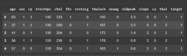
df = pd.read_csv('/content/heart.csv')
X = df.drop('target', axis=1)
y = df['target']
df.head()

Output:

3. Normalising the Features

We will normalize selected numeric features to scale them between 0 and 1.

• MinMaxScaler(): Initializes a Min-Max scaler.
• fit_transform(X[features]): Learns min and max values from data and scales features.
• X.copy(): Creates a copy to avoid modifying the original dataset.

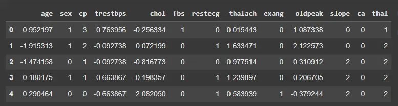
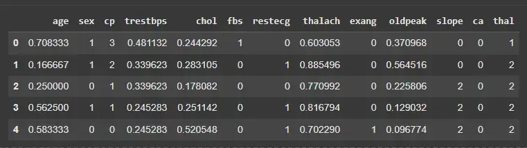
features = ['age','trestbps','chol','thalach','oldpeak']
scaler = MinMaxScaler()

X_normalized = X.copy()
X_normalized[features] = scaler.fit_transform(X[features])
X_normalized.head()

Output:

4. Standardizing the Features

We will standardize the same features to have mean 0 and standard deviation 1.

• StandardScaler(): Initializes a standard scaler.
• fit_transform(X[features]): Computes mean and standard deviation, then standardizes the features.

Note: Standardization is less sensitive to outliers compared to normalization.

scaler_z = StandardScaler()
X_standardized = X.copy()
X_standardized[features] = scaler_z.fit_transform(X[features])
X_standardized.head()

Output: