House Price Prediction – Data Understanding

Data Report

A data report communicates insights derived from data, not just numbers. A good report tells a logical, evidence-based story that supports decision-making.

Section	Main Goal
Title & Introduction	Define context and purpose
Business Logic	Explain why the analysis matters
Data Summary	Describe the dataset
Group & Sort	Show data organization logic
Visualizations	Communicate insights visually
Drill Down	Explore details and exceptions
Conclusions	Provide insights and actions
References	Support transparency
Footnotes	Give credit and clarifications

1. Title and Introduction

Set the context and tell the reader what the report is about and why it matters.

What to include

• Report title (clear and specific)
• Problem or question being addressed
• Scope of the analysis
• Target audience (business stakeholders, technical team, academics)

---

Title: House Price Prediction Analysis

Introduction:

• This report analyzes residential housing data to identify key factors influencing house prices and to support predictive modeling for pricing decisions.

2. Business Logic

Explain why the analysis exists from a business or real-world perspective.

What to include

• Business objectives
• Decision-making context
• How insights will be used
• Constraints or assumptions

---

Accurate house price prediction helps real estate agencies optimize pricing strategies and assists buyers in making informed investment decisions.

3. Data Summary

Help readers understand what data was used.

What to include

• Data sources
• Number of records and features
• Target variable
• Time period and coverage
• Basic data quality notes

---

Import CSV to SQLite

import pandas as pd
import sqlite3

# ==============================
# CONFIGURATION
# ==============================
CSV_PATH = "housing.csv"
DB_PATH = "housing.db"
TABLE_NAME = "houses"

# ==============================
# READ CSV
# ==============================
df = pd.read_csv(CSV_PATH)

# ==============================
# CONNECT TO SQLITE
# ==============================
conn = sqlite3.connect(DB_PATH)

# ==============================
# WRITE TO SQLITE
# ==============================
df.to_sql(
    TABLE_NAME,
    conn,
    if_exists="replace",  # overwrite table if exists
    index=False
)

# ==============================
# VERIFY INSERT
# ==============================
cursor = conn.cursor()
cursor.execute(f"SELECT COUNT(*) FROM {TABLE_NAME}")
row_count = cursor.fetchone()[0]

print(f"Imported {row_count:,} rows into table '{TABLE_NAME}'")

conn.close()

Anlysis data:

• Dataset: Housing market dataset
• Records: 25,000 properties
• Features: 18 variables (numeric and categorical)
• Target variable: House price

iimport sqlite3

# ==============================
# CONFIGURATION
# ==============================
DB_PATH = "housing.db"
TABLE_NAME = "houses"
DATASET_NAME = "Housing market dataset"
TARGET_VARIABLE = "price"

# ==============================
# CONNECT TO DATABASE
# ==============================
conn = sqlite3.connect(DB_PATH)
cursor = conn.cursor()

# ==============================
# NUMBER OF RECORDS
# ==============================
cursor.execute(f"SELECT COUNT(*) FROM {TABLE_NAME}")
num_records = cursor.fetchone()[0]

# ==============================
# NUMBER OF FEATURES (COLUMNS)
# ==============================
cursor.execute(f"PRAGMA table_info({TABLE_NAME})")
columns_info = cursor.fetchall()
num_features = len(columns_info)

# ==============================
# IDENTIFY NUMERIC VS CATEGORICAL
# ==============================
numeric_types = ("INT", "INTEGER", "REAL", "FLOAT", "DOUBLE")
numeric_count = 0
categorical_count = 0

for col in columns_info:
    col_type = col[2].upper()
    if any(t in col_type for t in numeric_types):
        numeric_count += 1
    else:
        categorical_count += 1

# ==============================
# OUTPUT DATA SUMMARY
# ==============================
print(f"Dataset: {DATASET_NAME}")
print(f"Records: {num_records:,} properties")
print(
    f"Features: {num_features} variables "
    f"({numeric_count} numeric, {categorical_count} categorical)"
)
print("Target variable: House price")

# ==============================
# CLOSE CONNECTION
# ==============================
conn.close()

4. Group By and Sort Criteria

Explain how data was aggregated or organized to reveal patterns.

What to include

• Grouping variables (e.g., location, year, category)
• Sorting logic (ascending, descending, top-k)
• Rationale for grouping

---

Data was grouped by district and sorted by average house price to identify high-value and low-value areas.

4.1. Grouping Variables

Trong pandas, grouping variables được truyền vào groupby().

df.groupby("district")
df.groupby("year")
df.groupby(["district", "house_type"])

4.2. Average House Price by District (Sort Descending)

avg_price_by_district = (
    df.groupby("district")["price"]
      .mean()
      .sort_values(ascending=False)
)

avg_price_by_district.head()

• Group by: district
• Metric: average price
• Sort: descending -> tìm khu vực giá cao

4.3 Group By + Multiple Aggregations (Best Practice)

district_summary = (
    df.groupby("district")
      .agg(
          avg_price=("price", "mean"),
          median_price=("price", "median"),
          num_properties=("price", "count")
      )
      .sort_values(by="avg_price", ascending=False)
)

district_summary.head()

4.4. Top-K Most Expensive Districts

top_5_districts = district_summary.head(5)
top_5_districts


Hoặc gộp trực tiếp:

top_5_districts = (
    df.groupby("district")["price"]
      .mean()
      .sort_values(ascending=False)
      .head(5)
)

4.5. Average Price Trend by Year (Sort Ascending)

price_trend_by_year = (
    df.groupby("year")["price"]
      .mean()
      .sort_index()
)

price_trend_by_year

• Sort theo năm tăng dần
• Dùng cho phân tích xu hướng

4.6. Group By Multiple Variables (District + House Type)

district_type_summary = (
    df.groupby(["district", "house_type"])
      .agg(
          avg_price=("price", "mean"),
          num_properties=("price", "count")
      )
      .sort_values(by="avg_price", ascending=False)
)

district_type_summary.head()

5. Visualizations

Make insights easy to understand and compare.

What to include

• Charts, graphs, and tables
• Clear titles and labels
• Explanation of what each visualization shows
• Best practices
• One insight per chart
• Avoid unnecessary decoration
• Always explain why the visualization matters

---

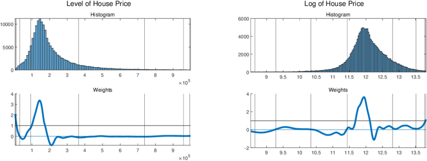
• Histogram of house prices

import matplotlib.pyplot as plt
import seaborn as sns

plt.figure(figsize=(8, 5))
sns.histplot(df['price'], bins=30, kde=True)

plt.title('Distribution of House Prices')
plt.xlabel('House Price')
plt.ylabel('Frequency')

plt.show()

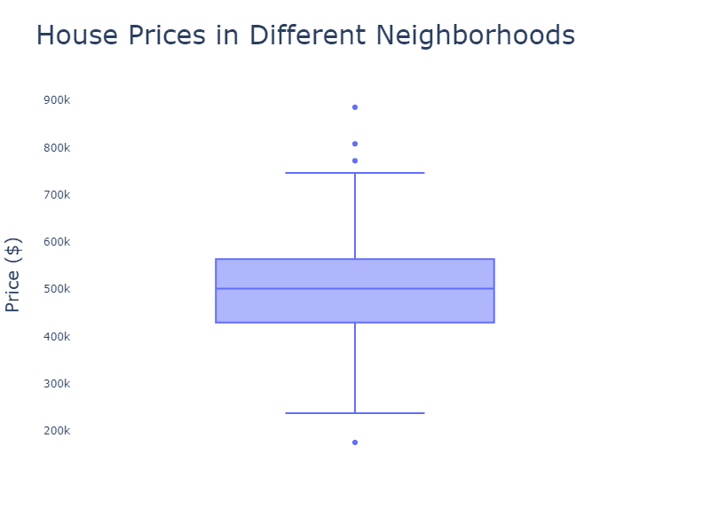
• Boxplot of prices by district

plt.figure(figsize=(10, 6))
sns.boxplot(x='district', y='price', data=df)

plt.title('House Prices by District')
plt.xlabel('District')
plt.ylabel('House Price')
plt.xticks(rotation=45)

plt.show()

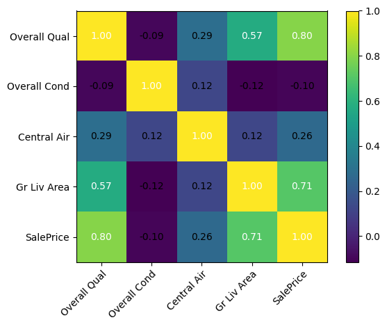
• Correlation heatmap of numeric features

import numpy as np

# Select numeric columns only
numeric_df = df.select_dtypes(include=np.number)

# Compute correlation matrix
corr_matrix = numeric_df.corr()

plt.figure(figsize=(10, 8))
sns.heatmap(
    corr_matrix,
    annot=True,
    fmt=".2f",
    cmap="coolwarm",
    square=True
)

plt.title('Correlation Heatmap of Numeric Features')
plt.show()

6. Drill Down

Allow deeper exploration of specific segments or anomalies.

What to include

• Subgroup analysis
• Focus on outliers or special cases
• Progressive levels of detail

---

After identifying District A as having the highest average prices, a drill-down analysis was conducted by house type and size.

Drill down analysis is the process of:

moving from high-level summaries to detailed views in order to understand why certain segments show unusual patterns or anomalies.

All houses
 └── District
      └── House type
           └── Individual properties / Outliers

Standard Drill Down Process (3 Steps)

Step 1: Identify Anomalies at a High Level

Question: Which groups show unusually high or low values?

district_summary = (
    df.groupby("district")
      .agg(
          avg_price=("price", "mean"),
          count=("price", "count")
      )
      .sort_values("avg_price", ascending=False)
)

district_summary.head()

High-level insight: District A has the highest average house price.

Step 2: Subgroup Analysis

Question: Within District A, which subgroups drive the high prices?

target_district = district_summary.index[0]

district_drill = (
    df[df["district"] == target_district]
      .groupby("house_type")
      .agg(
          avg_price=("price", "mean"),
          count=("price", "count")
      )
      .sort_values("avg_price", ascending=False)
)

district_drill

Intermediate insight: Apartments contribute most to the high prices in District A.

Step 3: Deep Drill Down (Outliers and Special Cases)

• 3.1 Detect Outliers Using the IQR Method

q1 = df["price"].quantile(0.25)
q3 = df["price"].quantile(0.75)
iqr = q3 - q1

outliers = df[
    (df["price"] < q1 - 1.5 * iqr) |
    (df["price"] > q3 + 1.5 * iqr)
]

outliers.head()

• 3.2 Outliers Within a Specific Subgroup

district_outliers = outliers[outliers["district"] == target_district]
district_outliers.sort_values("price", ascending=False).head()

Detailed insight: A small number of luxury properties significantly inflate the average price.

7. Conclusions and Recommendations

Translate analysis into actionable insights.

What to include

• Key findings (summarized)
• Business or practical implications
• Clear recommendations
• Limitations of the analysis

---

Larger living area and location are the strongest predictors of house price. Recommendation: prioritize these features in pricing models and valuation tools.

4-Step Process (Recommended)

Step 1: Summarize Key Findings

(What happened?)

• Select the 3–5 most important findings from the entire analysis.

Guidelines

• One key finding per sentence
• Focus on insights, not raw numbers
• Link each finding to the data analysis

Example

• Location is the strongest factor influencing house prices.
• Larger living areas are associated with higher prices.
• A small number of luxury properties significantly affect average prices in some districts.

Step 2: Explain Business or Practical Implications

(So what?)

Translate each finding into real-world meaning.

Guidelines

• Explain how the finding affects decisions or operations
• Avoid technical jargon
• Write from a stakeholder’s perspective

Example

• Pricing strategies should vary by location rather than using a single pricing rule.
• Average prices may be misleading in districts with extreme values.

Step 3: Provide Clear Recommendations

(What should be done?)

Convert insights into specific, actionable actions.

Guidelines

• Start each recommendation with an action verb
• Ensure recommendations are feasible
• Directly link recommendations to key findings

Example

• Prioritize location and living area as key features in price prediction models.
• Use median prices in addition to averages when reporting prices.
• Analyze luxury properties as a separate segment.

Step 4: State Limitations of the Analysis

(What should we be careful about?)

Acknowledge important constraints to ensure transparency and credibility.

Guidelines

• Mention 3–4 major limitations
• Be honest but concise
• Do not undermine the main conclusions

Example

• the dataset does not include macroeconomic factors such as interest rates.
• Some districts have limited data, which may affect result reliability.
• The analysis is based on historical data and may not reflect recent market changes.

8. References and Appendices

Ensure credibility, transparency, and reproducibility.

What to include

• Data sources
• External studies or documentation
• Appendices with detailed tables, formulas, or methods

---

• Data source documentation
• Model parameter settings
• Extended statistical tables

References
[1] Author, A. (Year). Title. Source.
[2] Kaggle. (2023). Housing Prices Dataset. https://www.kaggle.com/
[3] ...