Graph is a non-linear data structure like tree data structure. A Graph is composed of a set of vertices(V) and a set of edges(E). The vertices are connected with each other through edges.
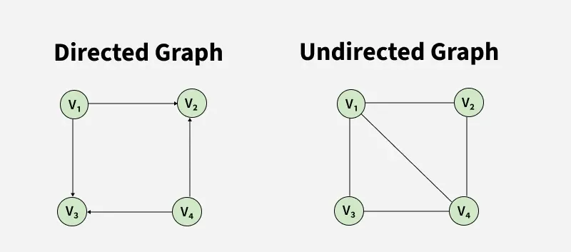
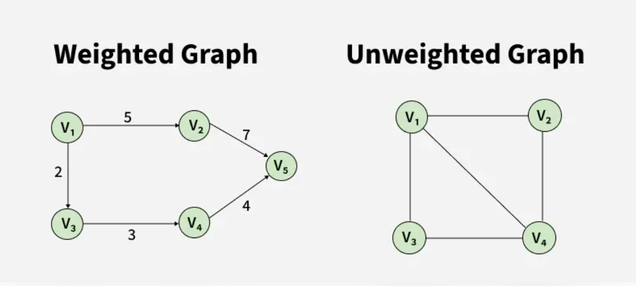
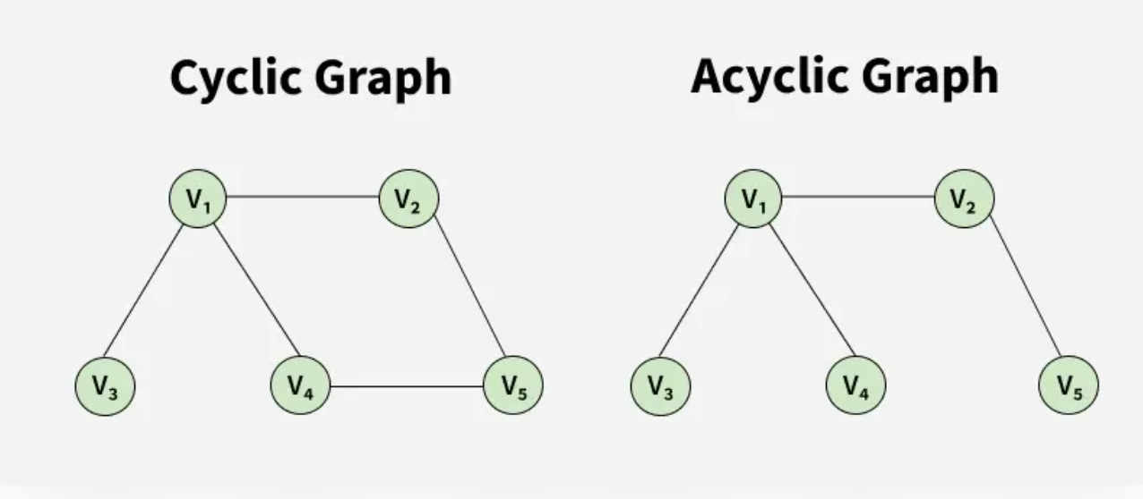
The following images show different types of graphs that see when solving graph problems.
Types:
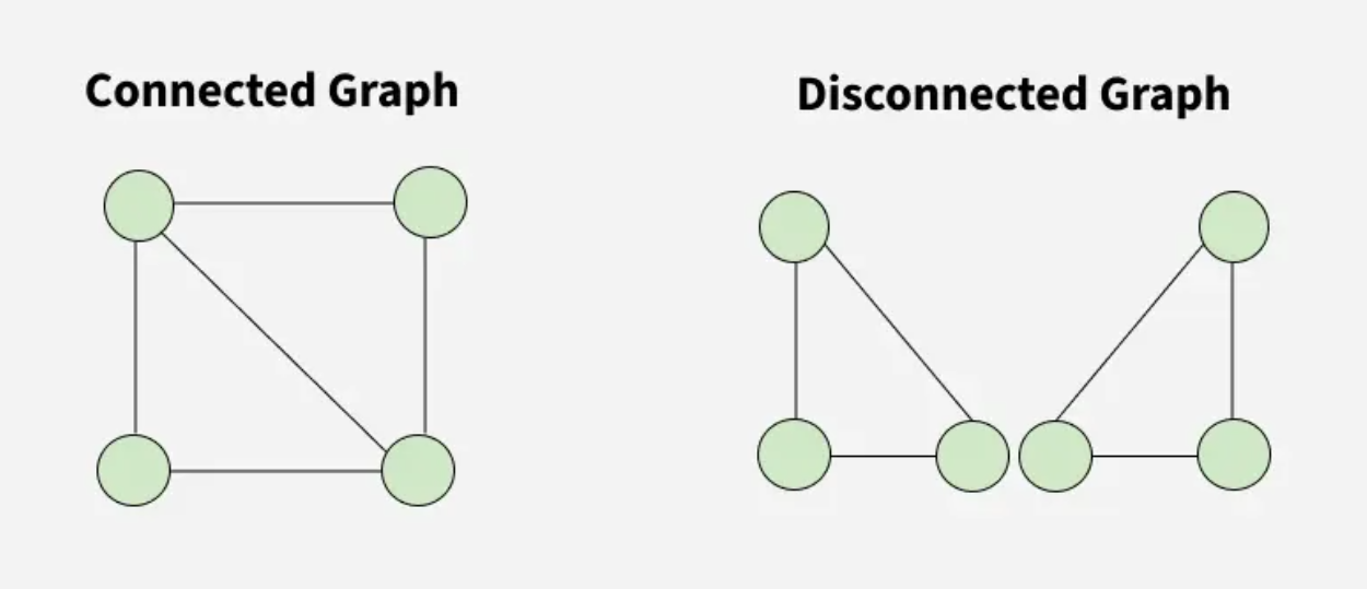
A Graph is a non-linear data structure consisting of vertices and edges. The vertices are sometimes also referred to as nodes and the edges are lines or arcs that connect any two nodes in the graph. More formally a Graph is composed of a set of vertices(V) and a set of edges(E). The graph is denoted by G(V, E).
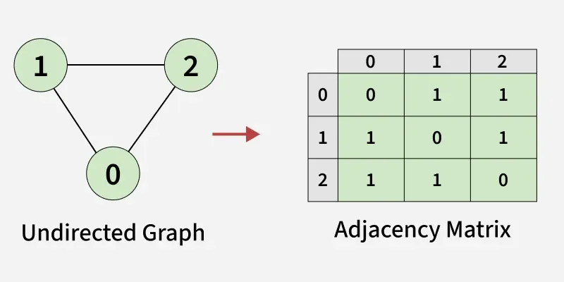
Here are the two most common ways to represent a graph : For simplicity, we are going to consider only unweighted graphs in this post.
An adjacency matrix is a way of representing a graph as a boolean matrix of (0’s and 1’s).
Let’s assume there are n vertices in the graph So, create a 2D matrix adjMat[n][n] having dimension n x n.
- If there is an edge from vertex i to j, mark adjMat[i][j] as 1.
- If there is no edge from vertex i to j, mark adjMat[i][j] as 0.
1
2
3
4
5
6
7
8
9
10
11
12
13
14
15
16
17
18
19
20
21
22
23
24
25
26
27
def createGraph(V, edges):
    mat = [[0 for _ in range(V)] for _ in range(V)]

    # Add each edge to the adjacency matrix
    for it in edges:
        u = it[0]
        v = it[1]
        mat[u][v] = 1

         # since the graph is undirected
        mat[v][u] = 1
    return mat

if __name__ == "__main__":
    V = 3

    # List of edges (u, v)
    edges = [[0, 1], [0, 2], [1, 2]]

    # Build the graph using edges
    mat = createGraph(V, edges)

    print("Adjacency Matrix Representation:")
    for i in range(V):
        for j in range(V):
            print(mat[i][j], end=" ")
        print()
Output
1
2
3
4
Adjacency Matrix Representation:
0 0 0
1 0 1
1 0 0
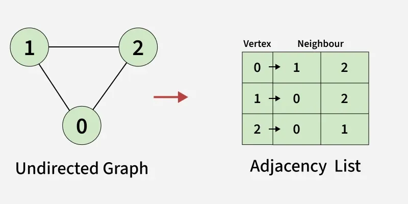
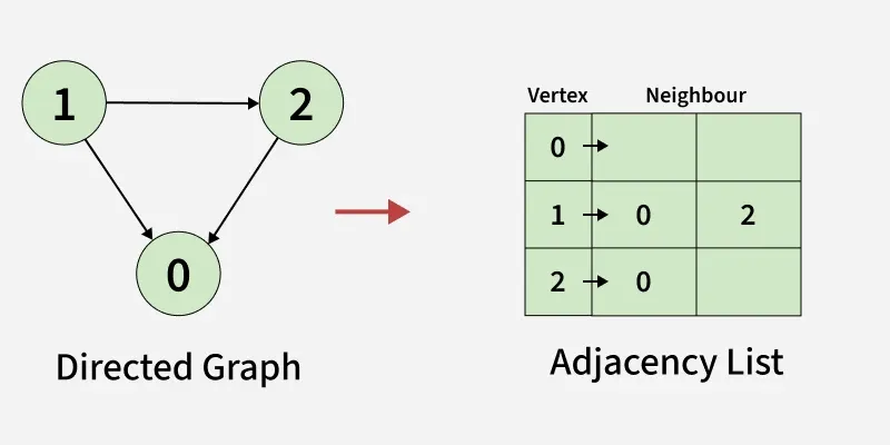
An array of Lists is used to store edges between two vertices. The size of array is equal to the number of vertices (i.e, n). Each index in this array represents a specific vertex in the graph. The entry at the index i of the array contains a linked list containing the vertices that are adjacent to vertex i. Let’s assume there are n vertices in the graph So, create an array of list of size n as adjList[n].
adjList[0] will have all the nodes which are connected (neighbour) to vertex 0. adjList[1] will have all the nodes which are connected (neighbour) to vertex 1 and so on.
1
2
3
4
5
6
7
8
9
10
11
12
13
14
15
16
17
18
19
20
21
22
23
24
25
26
27
28
29
30
31
32
33
def createGraph(V, edges):
    adj = [[] for _ in range(V)]

    # Add each edge to the adjacency list
    for it in edges:
        u = it[0]
        v = it[1]
        adj[u].append(v)

         # since the graph is undirected
        adj[v].append(u)
    return adj


if __name__ == "__main__":
    V = 3

    # List of edges (u, v)
    edges = [[0, 1], [0, 2], [1, 2]]

    # Build the graph using edges
    adj = createGraph(V, edges)

    print("Adjacency List Representation:")
    for i in range(V):

        # Print the vertex
        print(f"{i}:", end=" ")
        for j in adj[i]:

            # Print its adjacent
            print(j, end=" ")
        print()
Output
1
2
3
4
Adjacency List Representation:
0: 1 2
1: 0 2
2: 0 1
1
2
3
4
5
6
7
8
9
10
11
12
13
14
15
16
17
18
19
20
21
22
23
24
25
26
27
28
29
30
31
def createGraph(V, edges):
adj = [[] for _ in range(V)]
# Add each edge to the adjacency list
for it in edges:
u = it[0]
v = it[1]
adj[u].append(v)
return adj
if __name__ == "__main__":
V = 3
# List of edges (u, v)
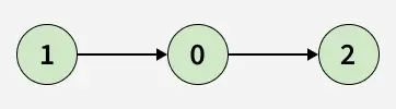
edges = [[1, 0], [1, 2], [2, 0]]
# Build the graph using edges
adj = createGraph(V, edges)
print("Adjacency List Representation:")
for i in range(V):
# Print the vertex
print(f"{i}:", end=" ")
for j in adj[i]:
# Print its adjacent
print(j, end=" ")
print()
Output
1
2
3
4
Adjacency List Representation:
0:
1: 0 2
2: 0
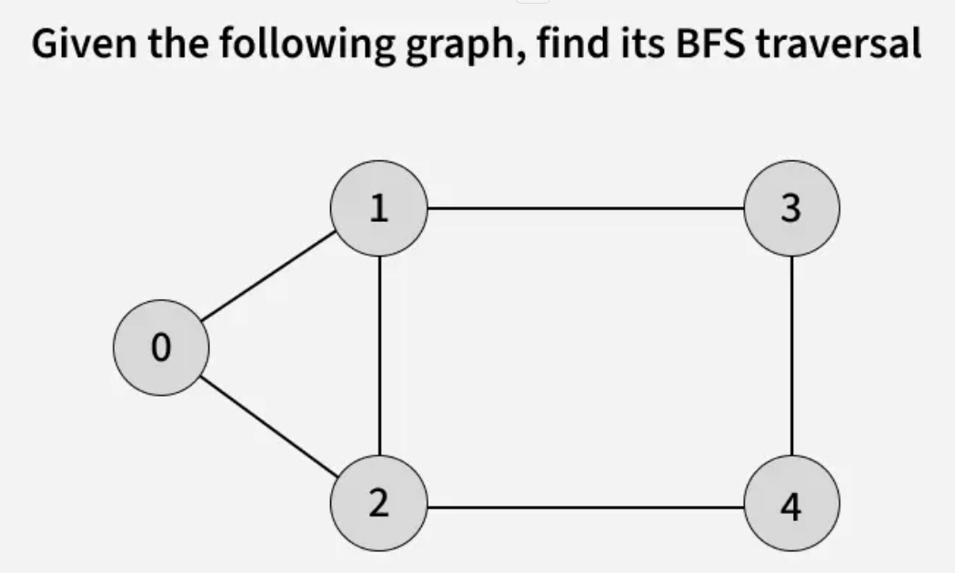
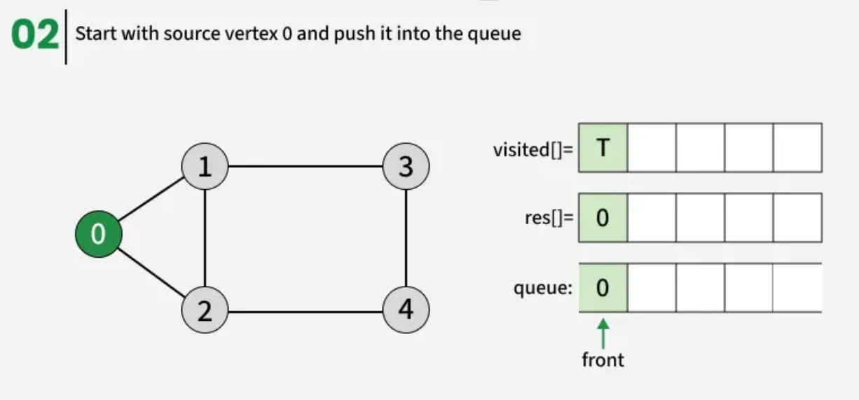
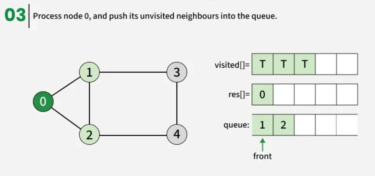
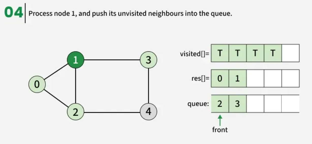
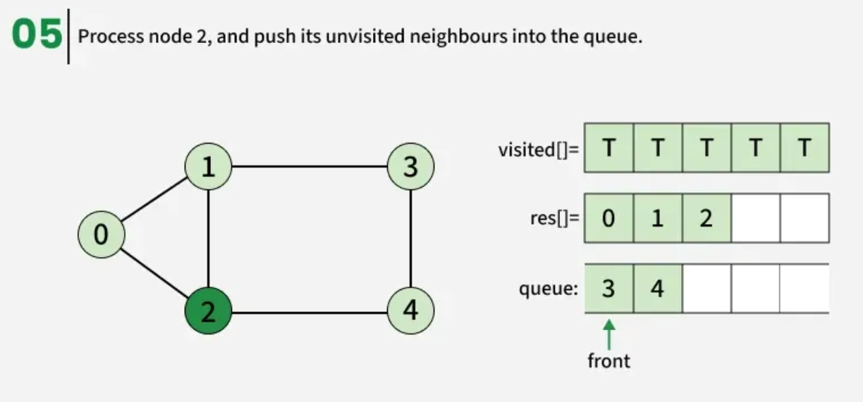
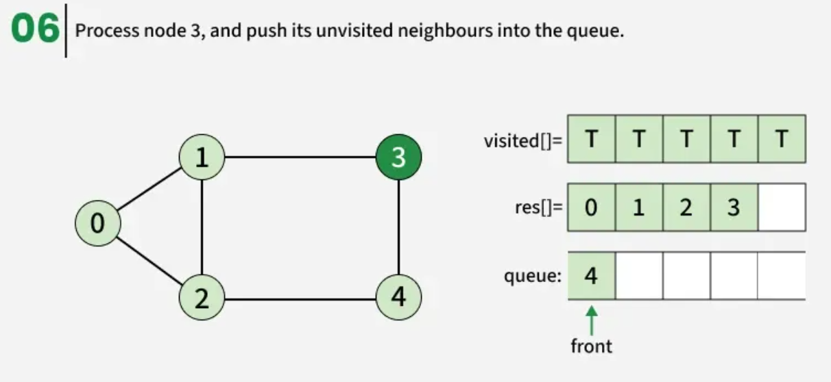
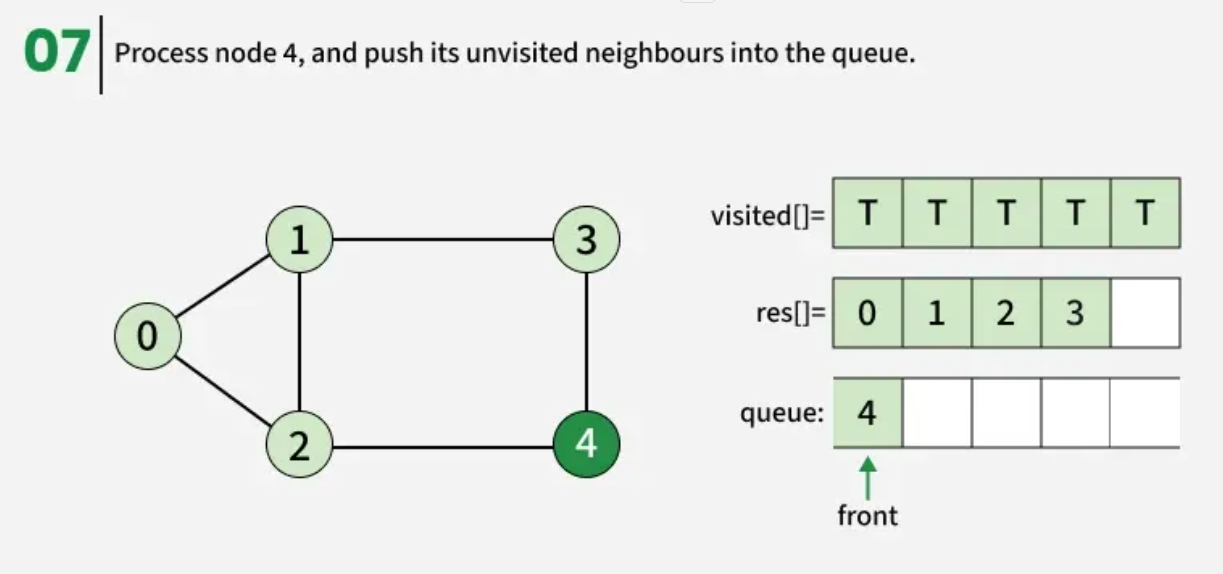
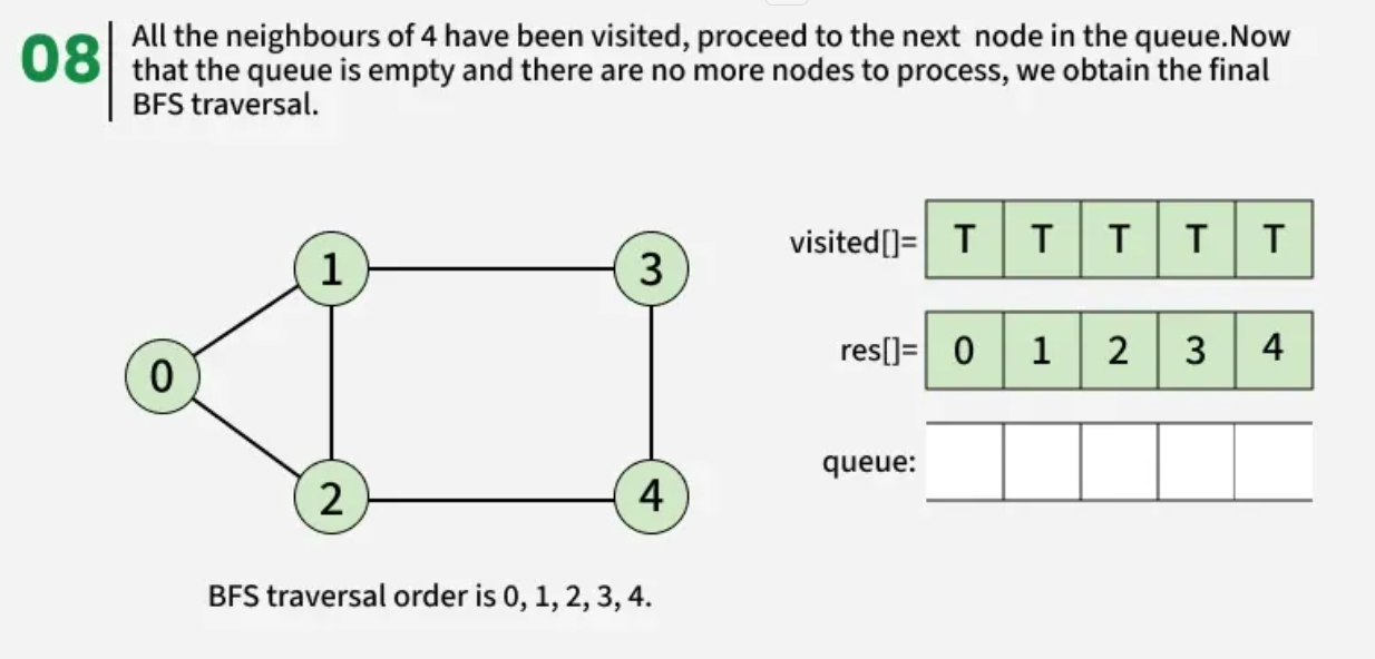
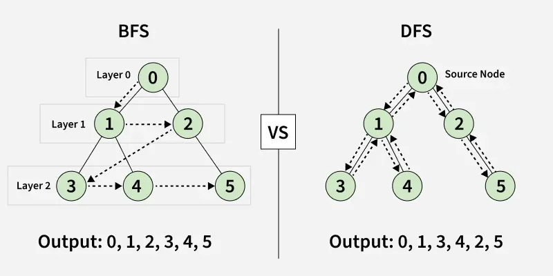
Breadth First Search (BFS) is a graph traversal algorithm that starts from a source node and explores the graph level by level. First, it visits all nodes directly adjacent to the source. Then, it moves on to visit the adjacent nodes of those nodes, and this process continues until all reachable nodes are visited.
Examples:
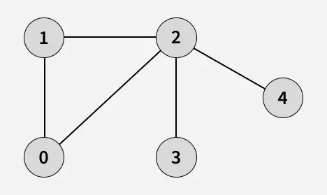
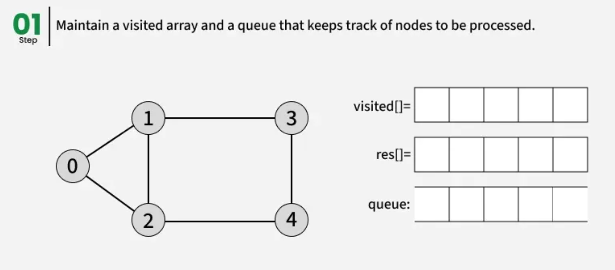
The algorithm starts from a given source vertex and explores all vertices reachable from that source, visiting nodes in increasing order of their distance from the source, level by level using a queue. Since graphs may contain cycles, a vertex could be visited multiple times. To prevent revisiting a vertex, a visited array is used.he working of Breadth First Search
The working of Breadth First Search
1
2
3
4
5
6
7
8
9
10
11
12
13
14
15
16
17
18
19
20
21
22
23
24
25
26
27
28
29
30
31
32
33
34
35
36
37
38
39
40
41
42
43
44
45
46
47
48
49
from collections import deque

# BFS for single connected component
def bfs(adj):
    V = len(adj)
    visited = [False] * V
    res = []

    src = 0
    q = deque()
    visited[src] = True
    q.append(src)

    while q:
        curr = q.popleft()
        res.append(curr)

        # visit all the unvisited
        # neighbours of current node
        for x in adj[curr]:
            if not visited[x]:
                visited[x] = True
                q.append(x)

    return res

def addEdge(adj, u, v):
    adj[u].append(v)
    adj[v].append(u)


if __name__ == "__main__":
    V = 5
    adj = []

    # creating adjacency list
    for i in range(V):
        adj.append([])

    addEdge(adj, 1, 2)
    addEdge(adj, 1, 0)
    addEdge(adj, 2, 0)
    addEdge(adj, 2, 3)
    addEdge(adj, 2, 4)

    res = bfs(adj)

    for node in res:
        print(node, end=" ")
Output
1
0 1 2 3 4
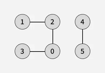
BFS of a Disconnected Undirected Graph:
In a disconnected graph, some vertices may not be reachable from a single source. To ensure all vertices are visited in BFS traversal, we iterate through each vertex, and if any vertex is unvisited, we perform a BFS starting from that vertex being the source. This way, BFS explores every connected component of the graph.
1
2
3
4
5
6
7
8
9
10
11
12
13
14
15
16
17
18
19
20
21
22
23
24
25
26
27
28
29
30
31
32
33
34
35
36
37
38
39
40
41
42
43
44
45
46
47
48
49
50
51
52
53
from collections import deque

# BFS for a single connected component
def bfsConnected(adj, src, visited, res):
    q = deque()
    visited[src] = True
    q.append(src)

    while q:
        curr = q.popleft()
        res.append(curr)

        # visit all the unvisited
        # neighbours of current node
        for x in adj[curr]:
            if not visited[x]:
                visited[x] = True
                q.append(x)

# BFS for all components (handles disconnected graphs)
def bfs(adj):
    V = len(adj)
    visited = [False] * V
    res = []

    for i in range(V):
        if not visited[i]:
            bfsConnected(adj, i, visited, res)
    return res

def addEdge(adj, u, v):
    adj[u].append(v)
    adj[v].append(u)


if __name__ == "__main__":
    V = 6
    adj = []

    # creating adjacency list
    for i in range(V):
        adj.append([])

    addEdge(adj, 1, 2)
    addEdge(adj, 2, 0)
    addEdge(adj, 0, 3)
    addEdge(adj, 4, 5)

    res = bfs(adj)

    for node in res:
        print(node, end=" ")
Output
1
0 2 3 1 4 5
Applications of BFS in Graphs
BFS has various applications in graph theory and computer science, including:
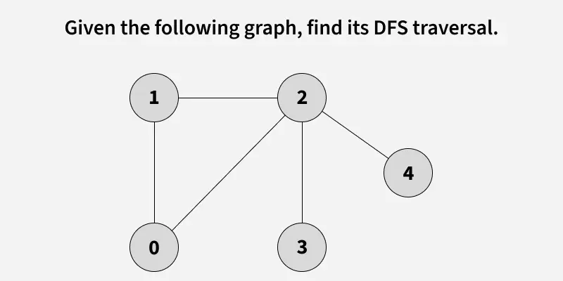
Given a graph, traverse the graph using Depth First Search and find the order in which nodes are visited.
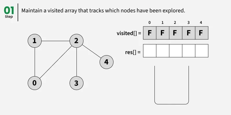
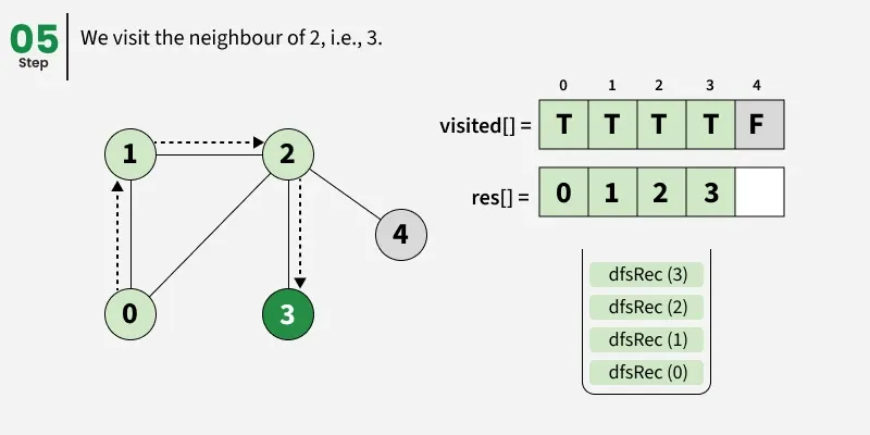
Depth First Search (DFS) is a graph traversal method that starts from a source vertex and explores each path completely before backtracking and exploring other paths. To avoid revisiting nodes in graphs with cycles, a visited array is used to track visited vertices.
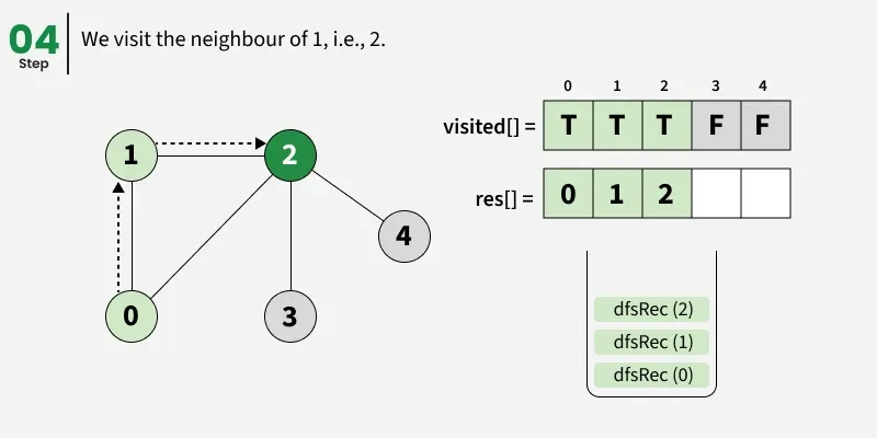
Note: There can be multiple DFS traversals of a graph according to the order in which we pick adjacent vertices. Here we pick vertices as per the insertion order.
Example:
Note that there can be more than one DFS Traversals of a Graph. For example, after 1, we may pick adjacent 2 instead of 0 and get a different DFS.
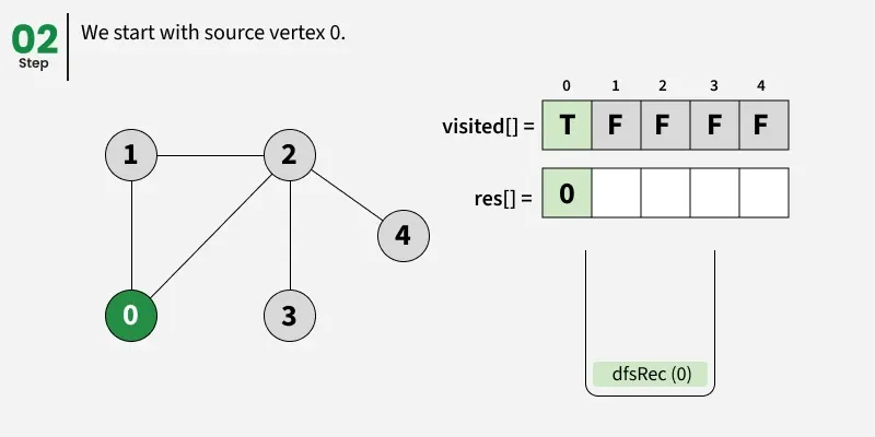
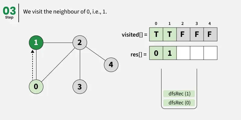
DFS from a Given Source of Graph:
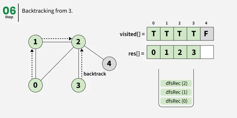
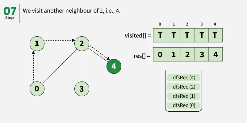
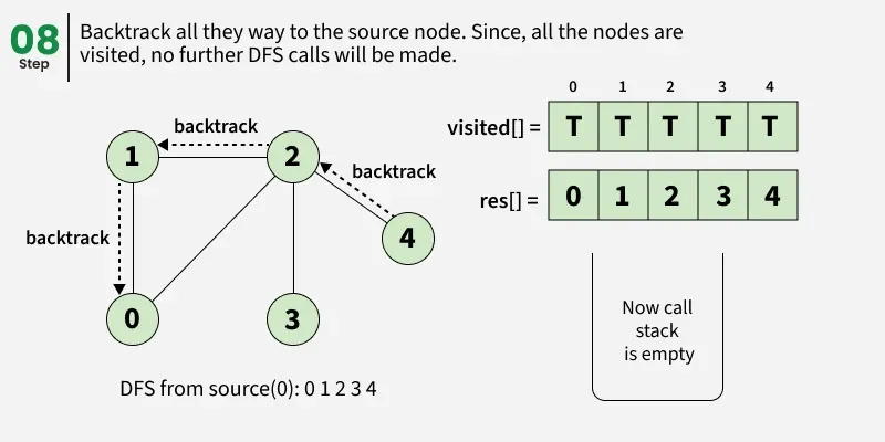
Depth First Search (DFS) starts from a given source vertex and explores one path as deeply as possible. When it reaches a vertex with no unvisited neighbors, it backtracks to the previous vertex to explore other unvisited paths. This continues until all vertices reachable from the source are visited. In a graph, there might be loops. So we use an extra visited array to make sure that we do not process a vertex again.
The working of Depth First Search:
1
2
3
4
5
6
7
8
9
10
11
12
13
14
15
16
17
18
19
20
21
22
23
24
25
26
27
28
29
30
31
32
33
34
35
36
37
38
39
40
41
def dfsRec(adj, visited, s, res):
    visited[s] = True
    res.append(s)

    # Recursively visit all adjacent vertices
    # that are not visited yet
    for i in adj[s]:
        if not visited[i]:
            dfsRec(adj, visited, i, res)


def dfs(adj):
    visited = [False] * len(adj)
    res = []
    dfsRec(adj, visited, 0, res)
    return res

def addEdge(adj, u, v):
    adj[u].append(v)
    adj[v].append(u)


if __name__ == "__main__":
    V = 5
    adj = []

    # creating adjacency list
    for i in range(V):
        adj.append([])

    addEdge(adj, 1, 2)
    addEdge(adj, 1, 0)
    addEdge(adj, 2, 0)
    addEdge(adj, 2, 3)
    addEdge(adj, 2, 4)

    # Perform DFS starting from vertex 0
    res = dfs(adj)

    for node in res:
        print(node, end=" ")
Output
1
0 1 2 3 4
DFS of a Disconnected Graph:
In a disconnected graph, some vertices may not be reachable from a single source. To ensure all vertices are visited in DFS traversal, we iterate through each vertex, and if a vertex is unvisited, we perform a DFS starting from that vertex being the source. This way, DFS explores every connected component of the graph.
1
2
3
4
5
6
7
8
9
10
11
12
13
14
15
16
17
18
19
20
21
22
23
24
25
26
27
28
29
30
31
32
33
34
35
36
37
38
39
40
41
42
43
44
45
46
from collections import defaultdict

def dfsRec(adj, visited, s, res):
    visited[s] = True
    res.append(s)

    # Recursively visit all adjacent
    # vertices that are not visited yet
    for i in adj[s]:
        if not visited[i]:
            dfsRec(adj, visited, i, res)


def dfs(adj):
    visited = [False] * len(adj)
    res = []
    # Loop through all vertices to
    # handle disconnected graph
    for i in range(len(adj)):
        if not visited[i]:
            dfsRec(adj, visited, i, res)
    return res

def addEdge(adj, u, v):
    adj[u].append(v)
    adj[v].append(u)


if __name__ == "__main__":
    V = 6
    adj = []

    # creating adjacency list
    for i in range(V):
        adj.append([])

    addEdge(adj, 1, 2)
    addEdge(adj, 2, 0)
    addEdge(adj, 0, 3)
    addEdge(adj, 5, 4)

    # Perform DFS
    res = dfs(adj)

    print(*res)
Output
1
0 3 2 1 4 5
Breadth-First Search (BFS) and Depth-First Search (DFS) are two fundamental algorithms used for traversing or searching graphs and trees. This article covers the basic difference between Breadth-First Search and Depth-First Search.
| Parameters | BFS | DFS |
|---|---|---|
| Stands for | BFS stands for Breadth First Search. | DFS stands for Depth First Search. |
| Data Structure | BFS (Breadth First Search) uses Queue data structure for finding the shortest path. | DFS (Depth First Search) uses Stack data structure. |
| Definition | BFS is a traversal approach in which we first walk through all nodes on the same level before moving on to the next level. | DFS is a traversal approach in which the traversal begins at the root node and proceeds through nodes as far as possible until reaching a node with no unvisited adjacent nodes. |
| Conceptual Difference | BFS builds the tree level by level. | DFS builds the tree sub-tree by sub-tree. |
| Approach used | It works on the concept of FIFO (First In First Out). | It works on the concept of LIFO (Last In First Out). |
| Suitable for | BFS is more suitable for searching vertices closer to the given source. | DFS is more suitable when solutions are far from the source. |
| Applications | BFS is used in applications such as bipartite graphs, shortest paths, etc. If every edge weight is the same, BFS gives the shortest path from source to every other vertex. | DFS is used in applications such as acyclic graphs and finding strongly connected components. Both BFS and DFS can also be used for Topological Sorting, Cycle Detection, etc. |
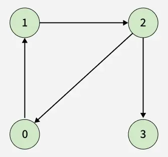
Given a directed graph represented by its adjacency list adj[][], determine whether the graph contains a cycle/Loop or not.
A cycle is a path that starts and ends at the same vertex, following the direction of edges.
Examples:
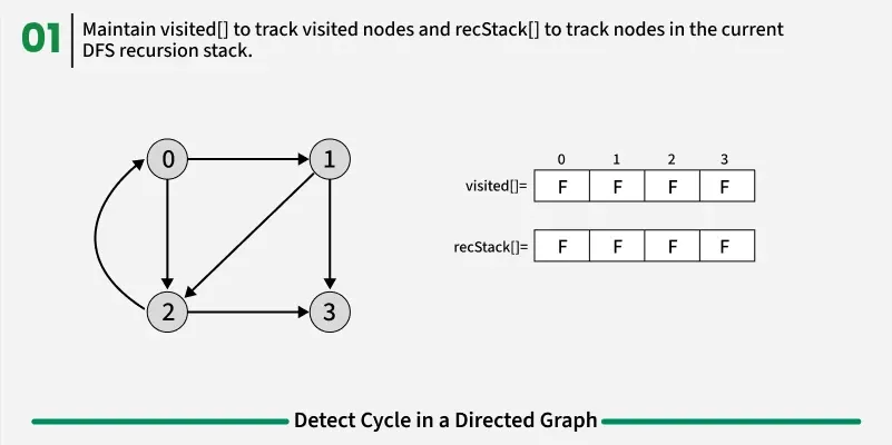
Detect Cycle algorithms
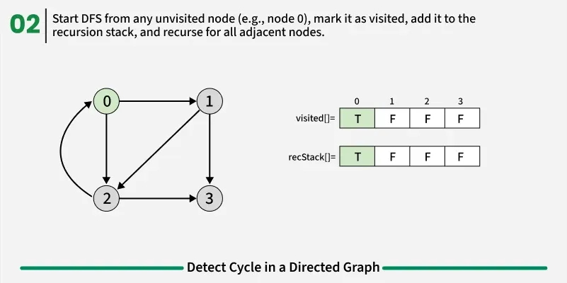
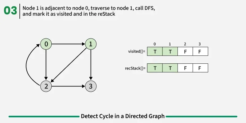
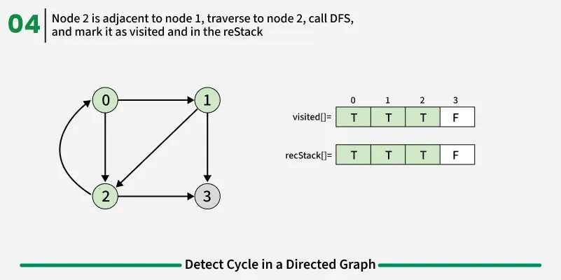
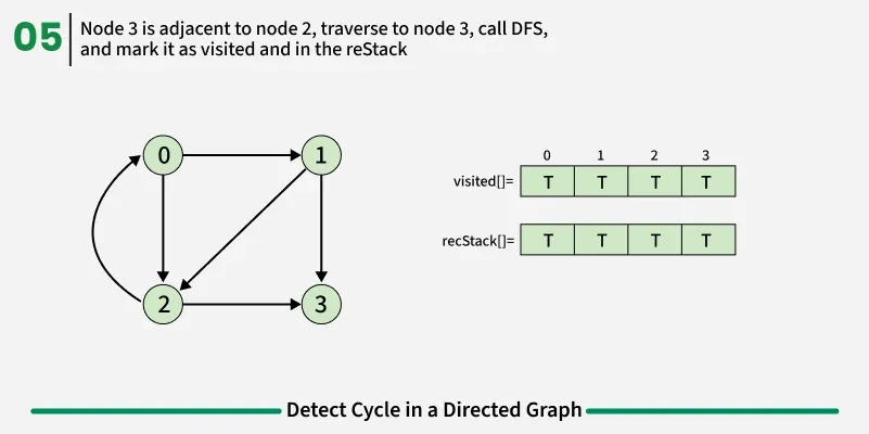
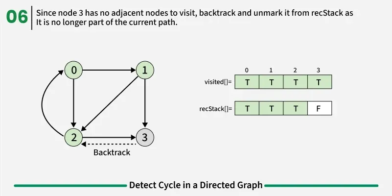
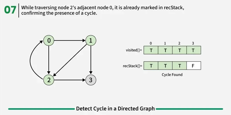
To detect a cycle in a directed graph, we use Depth First Search (DFS). In DFS, we go as deep as possible from a starting node. If during this process, we reach a node that we’ve already visited in the same DFS path, it means we’ve gone back to an ancestor — this shows a cycle exists. But there’s a problem: When we start DFS from one node, some nodes get marked as visited. Later, when we start DFS from another node, those visited nodes may appear again, even if there’s no cycle. So, using only visited[] isn’t enough.
To fix this, we use two arrays:
If during DFS we reach a node that’s already in the recStack, we’ve found a path from the current node back to one of its ancestors, forming a cycle. As soon as we finish exploring all paths from a node, we remove it from the recursion stack by marking recStack[node] = false. This ensures that only the nodes in the current DFS path are tracked.
1
2
3
4
5
6
7
8
9
10
11
12
13
14
15
16
17
18
19
20
21
22
23
24
25
26
27
28
29
30
31
32
33
34
35
36
37
38
39
40
# Utility DFS function to detect cycle in a directed graph
def isCyclicUtil(adj, u, visited, recStack):

    # node is already in recursion stack cycle found
    if recStack[u]:
        return True

    # already processed no need to visit again
    if visited[u]:
        return False

    visited[u] = True
    recStack[u] = True

    # Recur for all adjacent nodes
    for v in adj[u]:
        if isCyclicUtil(adj, v, visited, recStack):
            return True

    # remove from recursion stack before backtracking
    recStack[u] = False
    return False


# Function to detect cycle in a directed graph
def isCyclic(adj):
    V = len(adj)
    visited = [False] * V
    recStack = [False] * V

    # Run DFS from every unvisited node
    for i in range(V):
        if not visited[i] and isCyclicUtil(adj, i, visited, recStack):
            return True
    return False

if __name__ == "__main__":
    adj = [[1], [2], [0, 3]]

    print("true" if isCyclic(adj) else "false")
Output
1
true
The idea is to use Kahn’s algorithm because it works only for Directed Acyclic Graphs (DAGs). So, while performing topological sorting using Kahn’s algorithm, if we are able to include all the vertices in the topological order, it means the graph has no cycle and is a DAG. However, if at the end there are still some vertices left (i.e., their in-degree never becomes 0), it means those vertices are part of a cycle. Hence, if we cannot get all the vertices in the topological sort, the graph must contain at least one cycle.
1
2
3
4
5
6
7
8
9
10
11
12
13
14
15
16
17
18
19
20
21
22
23
24
25
26
27
28
29
30
31
32
33
34
35
36
37
38
39
40
41
from collections import deque

def isCyclic(adj):
    V = max(max(sub) if sub else 0 for sub in adj) + 1

    # Array to store in-degree of each vertex
    inDegree = [0] * V
    q = deque()

    # Count of visited (processed) nodes
    visited = 0

    # Compute in-degrees of all vertices
    for u in range(V):
        for v in adj[u]:
            inDegree[v] += 1

    # Add all vertices with in-degree 0 to the queue
    for u in range(V):
        if inDegree[u] == 0:
            q.append(u)

    # Perform BFS (Topological Sort)
    while q:
        u = q.popleft()
        visited += 1

        # Reduce in-degree of neighbors
        for v in adj[u]:
            inDegree[v] -= 1
            if inDegree[v] == 0:
                # Add to queue when in-degree becomes 0
                q.append(v)

    # If visited nodes != total nodes, a cycle exists
    return visited != V

if __name__ == "__main__":
    adj = [[1],[2],[0, 3], []]
    print("true" if isCyclic(adj) else "false")
Output
1
true
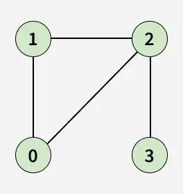
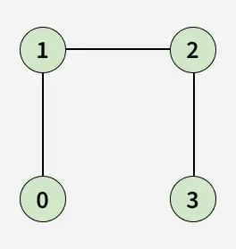
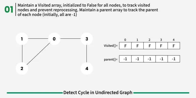
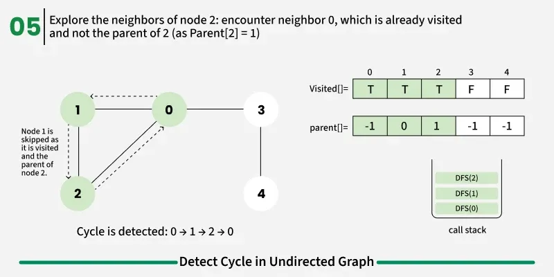
Given an adjacency list adj[][] representing an undirected graph, determine whether the graph contains a cycle/loop or not. A cycle is a path that starts and ends at the same vertex without repeating any edge.
Examples:
Detect Cycle algorithms
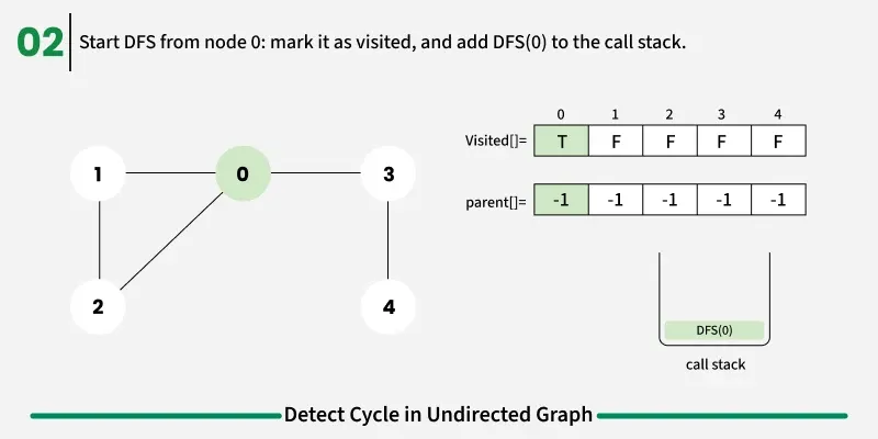
The idea is to use Depth First Search (DFS). When we start a DFS from a node, we visit all its connected neighbors one by one. If during this traversal, we reach a node that has already been visited before, it indicates that there might be a cycle, since we’ve come back to a previously explored vertex.
However, there’s one important catch.
In an undirected graph, every edge is bidirectional. That means, if there’s an edge from u -> v, then there’s also an edge from v -> u.
So, while performing DFS, from u, we go to v. From v, we again see u as one of its neighbors. Since u is already visited, it might look like a cycle — but it’s not.
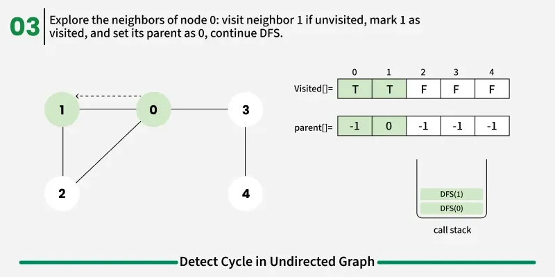
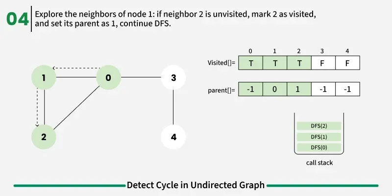
To avoid this issue, we keep track of the parent node — the node from which we reached the current node in DFS. When we move from u to v, we mark u as the parent of v. Now, while checking the neighbors of v, If a neighbor is not visited, we continue DFS for that node.If a neighbor is already visited and not equal to the parent, it means there’s another path that leads back to this node — and hence, a cycle exists.
1
2
3
4
5
6
7
8
9
10
11
12
13
14
15
16
17
18
19
20
21
22
23
24
25
26
27
28
29
30
31
32
33
34
35
36
37
38
39
def dfs(v, adj, visited, parent):

    # Mark the current node as visited
    visited[v] = True

    # Recur for all the vertices adjacent to this vertex
    for neighbor in adj[v]:

        # If an adjacent vertex is not visited,
        # then recur for that adjacent
        if not visited[neighbor]:
            if dfs(neighbor, adj, visited, v):
                return True

        # If an adjacent vertex is visited and is not
        # parent of current vertex,
        # then there exists a cycle in the graph.
        elif neighbor != parent:
            return True

    return False

# Returns true if the graph contains a cycle, else false.
def isCycle(adj):
    V = len(adj)
    # Mark all the vertices as not visited
    visited = [False] * V

    for u in range(V):
        if not visited[u]:
            if dfs(u, adj, visited, -1):
                return True

    return False

if __name__ == "__main__":
    adj = [[1, 2],[0, 2],[0, 1, 3],[2]]

    print("true" if isCycle(adj) else "false")
Output
1
true
The idea is quite similar to DFS-based cycle detection, but here we use Breadth First Search (BFS) instead of recursion. BFS explores the graph level by level, ensuring that each node is visited in the shortest possible way. It also helps avoid deep recursion calls, making it more memory-efficient for large graphs.
In BFS, we also maintain a visited array to mark nodes that have been explored and a parent tracker to remember from which node we reached the current one.
If during traversal we encounter a node that is already visited and is not the parent of the current node, it means we’ve found a cycle in the graph.
1
2
3
4
5
6
7
8
9
10
11
12
13
14
15
16
17
18
19
20
21
22
23
24
25
26
27
28
29
30
31
32
33
34
35
36
37
38
39
40
41
42
43
44
45
46
47
48
49
50
51
52
53
54
from collections import deque

# Function to perform BFS from node 'start' to detect cycle
def bfs(start, adj, visited):

    # Queue stores [current node, parent node]
    q = deque()

     # Start node has no parent
    q.append([start, -1])
    visited[start] = True

    while q:
        node = q[0][0]
        parent = q[0][1]
        q.popleft()

        # Traverse all neighbors of current node
        for neighbor in adj[node]:

            # If neighbor is not visited, mark it visited and push to queue
            if not visited[neighbor]:
                visited[neighbor] = True
                q.append([neighbor, node])
            # If neighbor is visited and not parent, a cycle is detected
            elif neighbor != parent:
                return True

    # No cycle found starting from this node
    return False

# Function to check if the undirected graph contains a cycle
def isCycle(adj):

    V = len(adj)

    # Keep track of visited vertices
    visited = [False] * V

    # Perform BFS from every unvisited node
    for i in range(V):
        if not visited[i]:

            # If BFS finds a cycle
            if bfs(i, adj, visited):
                return True

    # If no cycle is found in any component
    return False

if __name__ == "__main__":
    adj = [[1, 2],[0, 2],[0, 1, 3],[2]]

    print("true" if isCycle(adj) else "false")
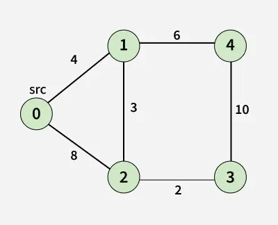
Given a weighted undirected graph and a source vertex src. We need to find the shortest path distances from the source vertex to all other vertices in the graph.
Note: The given graph does not contain any negative edge.
Examples:
1
2
3
4
5
Input: src = 0, adj[][] = [[[1, 4], [2, 8]],
                        [[0, 4], [4, 6], [2,3]],
                        [[0, 8], [3, 2], [1,3]],
                        [[2, 2], [4, 10]],
                        [[1, 6], [3, 10]]]
1
2
3
4
5
6
7
Output:  [0, 4, 7, 9, 10]
Explanation:  Shortest Paths:
- 0 -> 0 = 0: Source node itself, so distance is 0.
- 0 -> 1 = 4: Direct edge from node 0 to 1 gives shortest distance 4.
- 0 -> 2 = 7: Path 0 -> 1 -> 2 gives total cost 4 + 3 = 7, which is smaller than direct edge 8.
- 0 -> 3 = 9: Path 0 -> 1 -> 2 -> 3 gives total cost 4 + 3 + 2 = 9.
- 0 -> 4 = 10: Path 0 -> 1 -> 4 gives total cost 4 + 6 = 10.
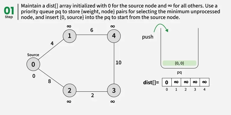
The idea is to maintain distance using an array dist[] from the given source to all vertices. The distance array is initialized as infinite for all vertexes and 0 for the given source We also maintain two sets,
- One set contains vertices included in the shortest-path tree,
- The other set includes vertices not yet included in the shortest-path tree.
At every step of the algorithm, find a vertex that is in the other set (set not yet included) and has a minimum distance from the source. Once we pick a vertex, we update the distance of its adjacent if we get a shorter path through it.
Use of priority Queue
The priority queue always selects the node with the smallest current distance, ensuring that we explore the shortest paths first and avoid unnecessary processing of longer paths. Dijkstra’s algorithm always picks the node with the minimum distance first. By doing so, it ensures that the node has already checked the shortest distance to all its neighbors. If this node appears again in the priority queue later, we don’t need to process it again, because its neighbors have already checked the minimum possible distances
Detailed Steps:
Trace solutions
1
2
3
4
5
6
7
8
while (Unvisited ≠ ∅)
    currNode = vertex có distance nhỏ nhất
    for mỗi đỉnh kề v của currNode
        newDistance = distance(currNode) + edgeWeight(currNode,v)
        if newDistance < distance(v)
            distance(v) = newDistance
            parent(v) = currNode
    Visited = Visited ∪ {currNode}
| Step | Current Node | 0 | 1 | 2 | 3 | 4 |
|---|---|---|---|---|---|---|
| 0 | - | {0,-} | {∞,-} | {∞,-} | {∞,-} | {∞,-} |
| 1 | 0 | {0,-} | {4,0} | {8,0} | {∞,-} | {∞,-} |
| 2 | 1 | {0,-} | {4,0} | {8,0} | {∞,-} | {10,1} |
| 3 | 2 | {0,-} | {4,0} | {8,0} | {10,2} | {10,1} |
| 4 | 3 | {0,-} | {4,0} | {8,0} | {10,2} | {10,1} |
| 5 | 4 | {0,-} | {4,0} | {8,0} | {10,2} | {10,1} |
Dijkstra’s Algorithm Trace
| Step | Current Node | Distance Table ({distance, parent}) |
Priority Queue (Min -> Max) |
|---|---|---|---|
| 0 | - | 0:{0,-} 1:{∞,-} 2:{∞,-} 3:{∞,-} 4:{∞,-} | {(0,0)} |
| 1 | 0 | 0:{0,-} 1:{4,0} 2:{8,0} 3:{∞,-} 4:{∞,-} | {(4,1), (8,2)} |
| 2 | 1 | 0:{0,-} 1:{4,0} 2:{8,0} 3:{∞,-} 4:{10,1} | {(8,2), (10,4)} |
| 3 | 2 | 0:{0,-} 1:{4,0} 2:{8,0} 3:{10,2} 4:{10,1} | {(10,3), (10,4)} |
| 4 | 3 | 0:{0,-} 1:{4,0} 2:{8,0} 3:{10,2} 4:{10,1} | {(10,4)} |
| 5 | 4 | 0:{0,-} 1:{4,0} 2:{8,0} 3:{10,2} 4:{10,1} | {} |
| 6 | Finish | Final distances: 0:{0,-} 1:{4,0} 2:{8,0} 3:{10,2} 4:{10,1} | Empty |
Step 0 – Initialization
Initialize the distance table.
1
2
3
4
5
dist[0] = 0
dist[1] = ∞
dist[2] = ∞
dist[3] = ∞
dist[4] = ∞
Initialize the priority queue.
1
pq = {(0,0)}
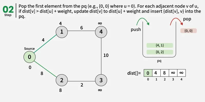
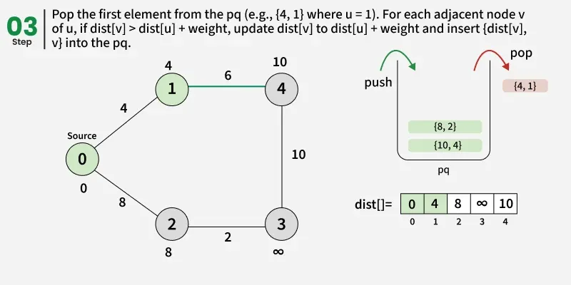
Step 1
1
2
Pop: {0,0}
Current Node = 0
Relax adjacent vertices.
1
2
3
4
5
0 -> 1
newDistance = 0 + 4 = 4
Update:
1 = {4,0}
Push {4,1}
1
2
3
4
5
0 -> 2
newDistance = 0 + 8 = 8
Update:
2 = {8,0}
Push {8,2}
Priority Queue
1
{(4,1), (8,2)}
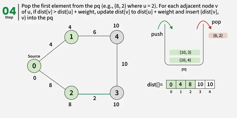
Step 2
1
2
Pop: {4,1}
Current Node = 1
Relax adjacent vertices.
1
2
3
4
5
1 -> 4
newDistance = 4 + 6 = 10
Update:
4 = {10,1}
Push {10,4}
Priority Queue
1
{(8,2), (10,4)}
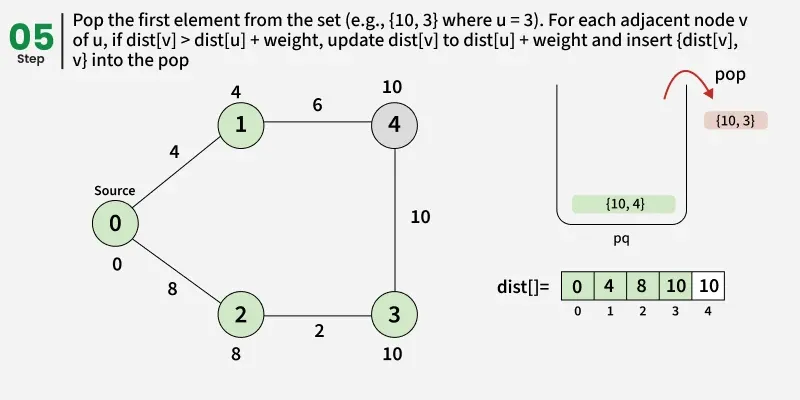
Step 3
1
2
Pop: {8,2}
Current Node = 2
Relax adjacent vertices.
1
2
3
4
5
2 -> 3
newDistance = 8 + 2 = 10
Update:
3 = {10,2}
Push {10,3}
Priority Queue
1
{(10,3), (10,4)}
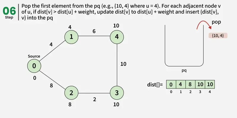
Step 4
1
2
Pop: {10,3}
Current Node = 3
Relax adjacent vertices.
1
2
3
4
3 -> 4
newDistance = 10 + 10 = 20
20 > 10
No update
Priority Queue
1
{(10,4)}
Step 5
1
2
Pop: {10,4}
Current Node = 4
Relax adjacent vertices.
1
2
3
4
4 -> 3
newDistance = 10 + 10 = 20
20 > 10
No update
Priority Queue
1
{}
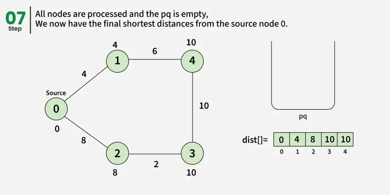
Step 6 – Finish
The priority queue is empty.
The final shortest distances from the source vertex are
| Vertex | {Distance, Parent} | Shortest Path |
|---|---|---|
| 0 | {0,-} | 0 |
| 1 | {4,0} | 0 -> 1 |
| 2 | {8,0} | 0 -> 2 |
| 3 | {10,2} | 0 -> 2 -> 3 |
| 4 | {10,1} | 0 -> 1 -> 4 |
1
2
3
4
5
6
7
8
9
10
11
12
13
14
15
16
17
18
19
20
21
22
23
24
25
26
27
28
29
30
31
32
33
34
35
36
37
38
39
40
41
42
43
44
45
46
47
48
49
import heapq
import sys

def dijkstra(adj, src):

    V = len(adj)

    # Min-heap (priority queue) storing pairs of (distance, node)
    pq = []

    dist = [sys.maxsize] * V

    # Distance from source to itself is 0
    dist[src] = 0
    heapq.heappush(pq, (0, src))

    # Process the queue until all reachable vertices are finalized
    while pq:
        d, u = heapq.heappop(pq)

        # If this distance not the latest shortest one, skip it
        if d > dist[u]:
            continue

        # Explore all neighbors of the current vertex
        for v, w in adj[u]:

            # If we found a shorter path to v through u, update it
            if dist[u] + w < dist[v]:
                dist[v] = dist[u] + w
                heapq.heappush(pq, (dist[v], v))

    # Return the final shortest distances from the source
    return dist

if __name__ == "__main__":
    src = 0

    adj = [
        [(1, 4), (2, 8)],
        [(0, 4), (4, 6), (2, 3)],
        [(0, 8), (3, 2), (1, 3)],
        [(2, 2), (4, 10)],
        [(1, 6), (3, 10)]
    ]

    result = dijkstra(adj, src)
    print(*result)
Output
1
0 4 7 9 10
Limitation of Dijkstra’s Algorithm:
Since, we need to find the single source shortest path, we might initially think of using Dijkstra’s algorithm. However, Dijkstra is not suitable when the graph consists of negative edges. The reason is, it doesn’t revisit those nodes which have already been marked as visited. If a shorter path exists through a longer route with negative edges, Dijkstra’s algorithm will fail to handle it.
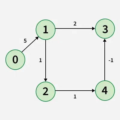
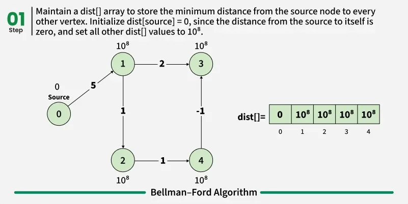
Given a weighted graph with V vertices and E edges, along with a source vertex src, the task is to compute the shortest distances from the source to all other vertices. If a vertex is unreachable from the source, its distance should be marked as 10^8. In the presence of a negative weight cycle, return -1 to signify that shortest path calculations are not feasible.
Examples:
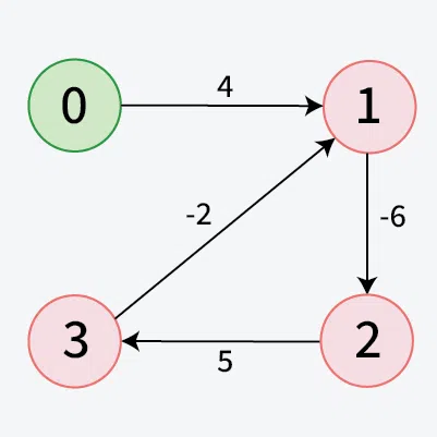
Detection of a Negative Weight Cycle
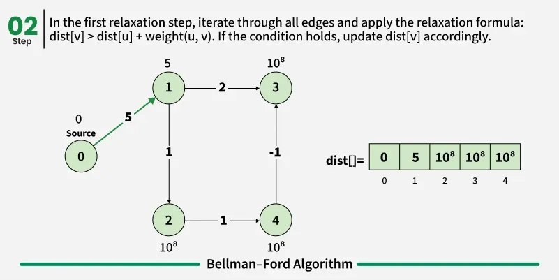
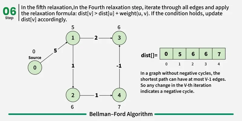
As we have discussed earlier that, we need (V - 1) relaxations of all the edges to achieve single source shortest path. If one additional relaxation (Vth) for any edge is possible, it indicates that some edges with overall negative weight has been traversed once more. This indicates the presence of a negative weight cycle in the graph.
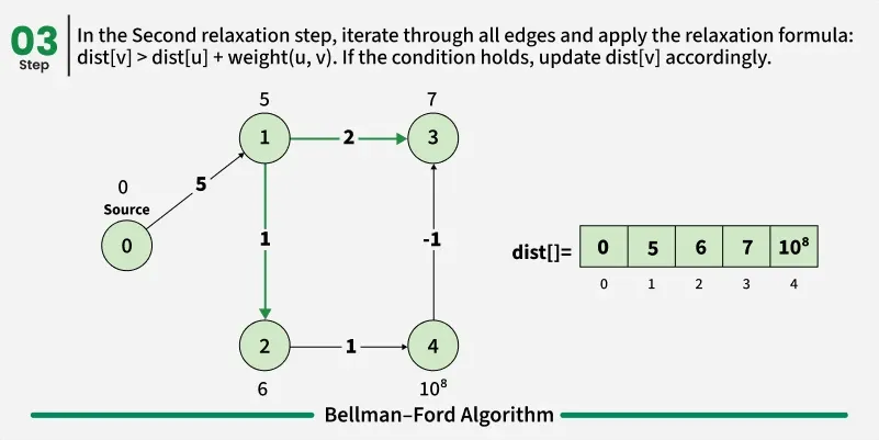
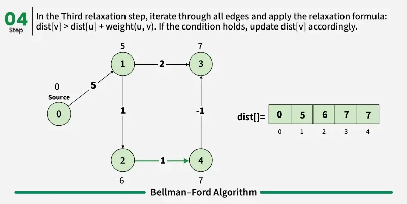
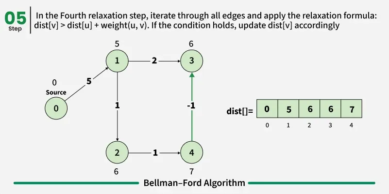
Bellman-Ford is a single source shortest path algorithm. It effectively works in the cases of negative edges and is able to detect negative cycles as well. It works on the principle of relaxation of the edges.
1
2
3
4
5
6
7
8
9
10
11
12
13
14
15
16
17
18
19
20
21
22
23
24
25
26
27
28
29
30
def bellmanFord(V, edges, src):

    # Initially distance from source to all other vertices
    # is not known(Infinite) e.g. 1e8.
    dist = [100000000] * V
    dist[src] = 0

    # Relaxation of all the edges V times, not (V - 1) as we
    # need one additional relaxation to detect negative cycle
    for i in range(V):
        for edge in edges:
            u, v, wt = edge
            if dist[u] != 100000000 and dist[u] + wt < dist[v]:

                # If this is the Vth relaxation, then there
                # is a negative cycle
                if i == V - 1:
                    return [-1]

                # Update shortest distance to node v
                dist[v] = dist[u] + wt
    return dist

if __name__ == '__main__':
    V = 5
    edges = [[1, 3, 2], [4, 3, -1], [2, 4, 1], [1, 2, 1], [0, 1, 5]]

    src = 0
    ans = bellmanFord(V, edges, src)
    print(' '.join(map(str, ans)))
Output
1
0 5 6 6 7
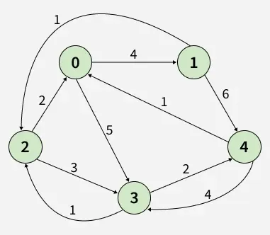
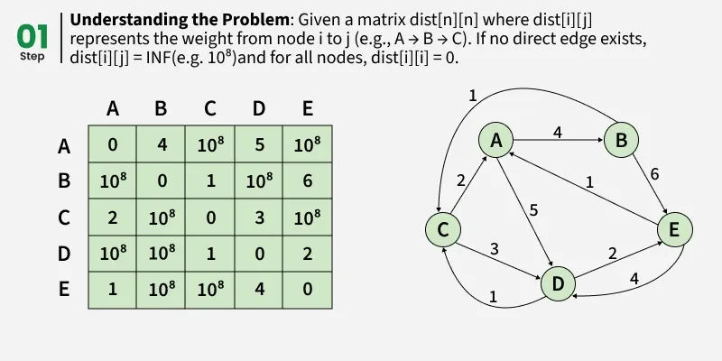
Given a matrix dist[][] of size n x n, where dist[i][j] represents the weight of the edge from node i to node j.
Determine the shortest path distance between all pair of nodes in the graph.
Example:
1
2
3
4
5
Input: dist[][] = [[0, 4, INF, 5, INF],
                [INF, 0, 1, INF, 6],
                [2, INF, 0, 3, INF],
                [INF, INF, 1, 0, 2],
                [1, INF, INF, 4, 0]]
1
2
3
4
5
6
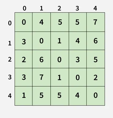
Output:[[0, 4, 5, 5, 7],
[3, 0, 1, 4, 6],
[2, 6, 0, 3, 5],
[3, 7, 1, 0, 2],
[1, 5, 5, 4, 0]]
Explanation:
1
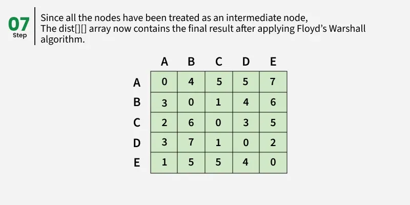
Each cell dist[i][i] in the output shows the shortest distance from node i to node j, computed by considering all possible intermediate nodes using the Floyd-Warshall algorithm.
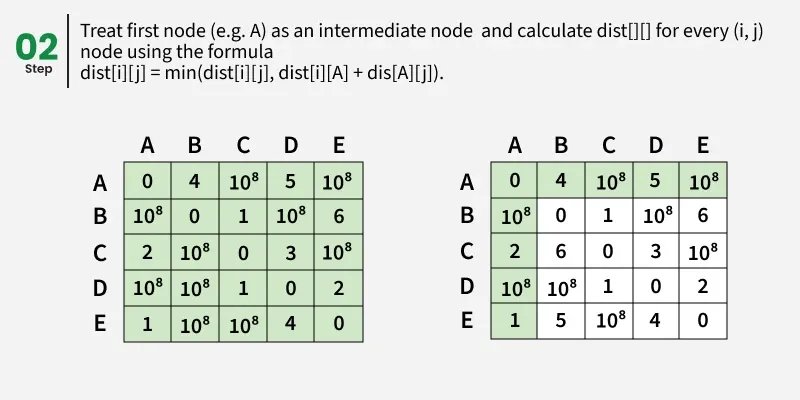
Floyd Warshall Algorithm:
The Floyd–Warshall algorithm works by maintaining a two-dimensional array that represents the distances between nodes. Initially, this array is filled using only the direct edges between nodes. Then, the algorithm gradually updates these distances by checking if shorter paths exist through intermediate nodes.
This algorithm works for both the directed and undirected weighted graphs and can handle graphs with both positive and negative weight edges.
Note: It does not work for the graphs with negative cycles (where the sum of the edges in a cycle is negative).
Suppose we have a graph dist[][] with V vertices from 0 to V-1. Now we have to evaluate a dist[][] where dist[i][j] represents the shortest path between vertex i to j.
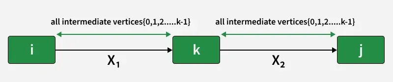
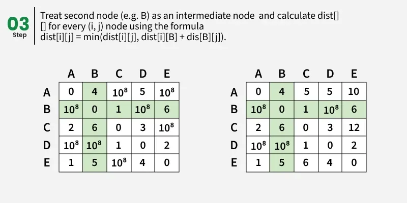
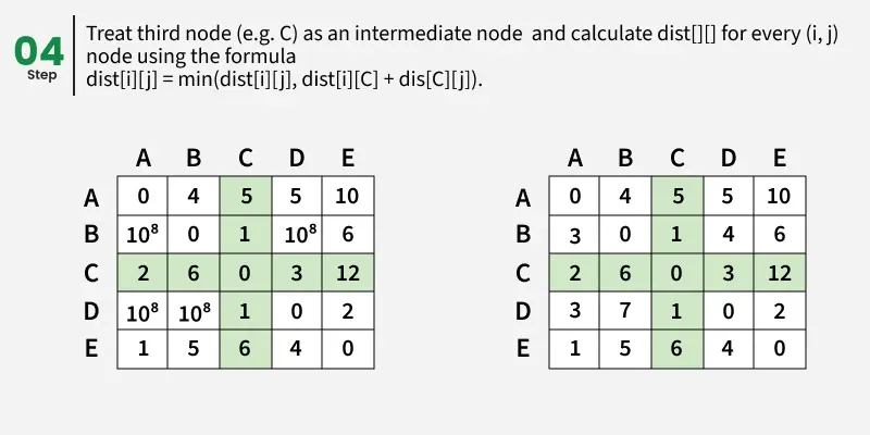
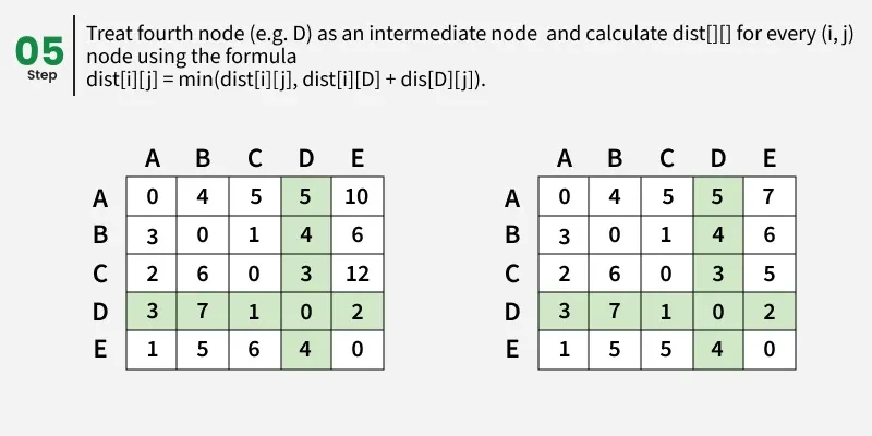
Let us assume that vertices i to j have intermediate nodes. The idea behind Floyd Warshall algorithm is to treat each and every vertex k from 0 to V-1 as an intermediate node one by one. When we consider the vertex k, we must have considered vertices from 0 to k-1 already. So we use the shortest paths built by previous vertices to build shorter paths with vertex k included.
The following figure shows the above optimal substructure property in Floyd Warshall algorithm:
Step-by-step implementation

1
2
3
4
5
6
7
8
9
10
11
12
13
14
15
16
17
18
19
20
21
22
23
24
25
26
27
28
29
30
31
def floydWarshall(dist):
    V = len(dist)
    INF = int(1e8)

    # for each intermediate vertex
    for k in range(V):

        # Pick all vertices as source one by one
        for i in range(V):

            # Pick all vertices as destination
            # for the above picked source
            for j in range(V):

                # shortest path from i to j
                if dist[i][k] != INF and dist[k][j] != INF:
                    dist[i][j] = min(dist[i][j],
                                     dist[i][k] + dist[k][j])

if __name__ == "__main__":
    INF = int(1e8)
    dist = [[0, 4, INF, 5, INF],
            [INF, 0, 1, INF, 6],
            [2, INF, 0, 3, INF],
            [INF, INF, 1, 0, 2],
            [1, INF, INF, 4, 0]]

    floydWarshall(dist)

    for row in dist:
        print(*row)
Output
1
2
3
4
5
0 4 5 5 7
3 0 1 4 6
2 6 0 3 5
3 7 1 0 2
1 5 5 4 0
Applications of Floyd-Warshall Algorithm:
Prim’s algorithm is a Greedy algorithm like Kruskal’s algorithm. This algorithm always starts with a single node and moves through several adjacent nodes, in order to explore all of the connected edges along the way.
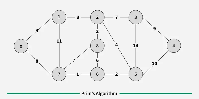
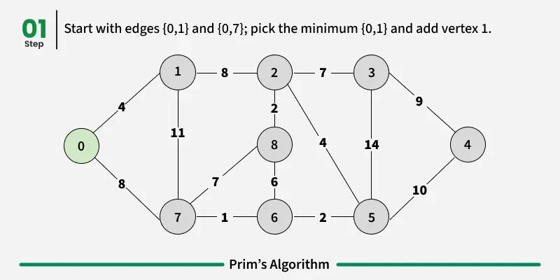
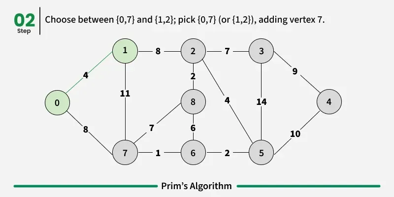
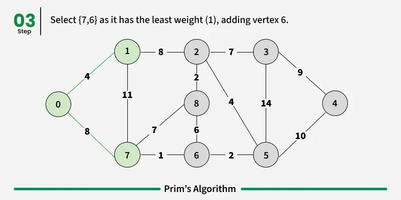
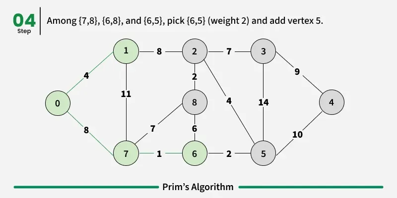
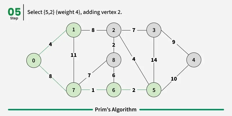
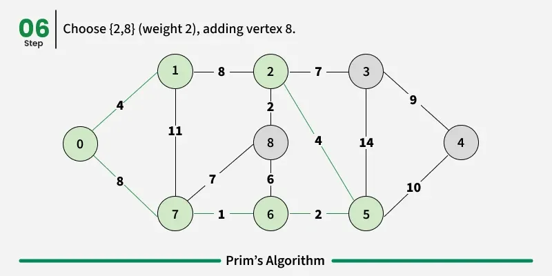
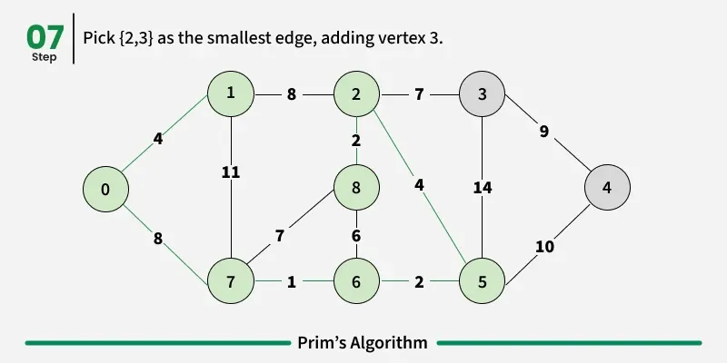
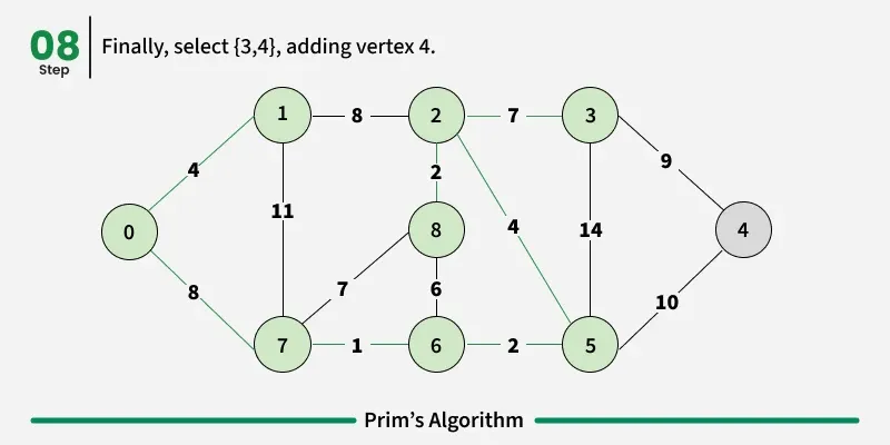
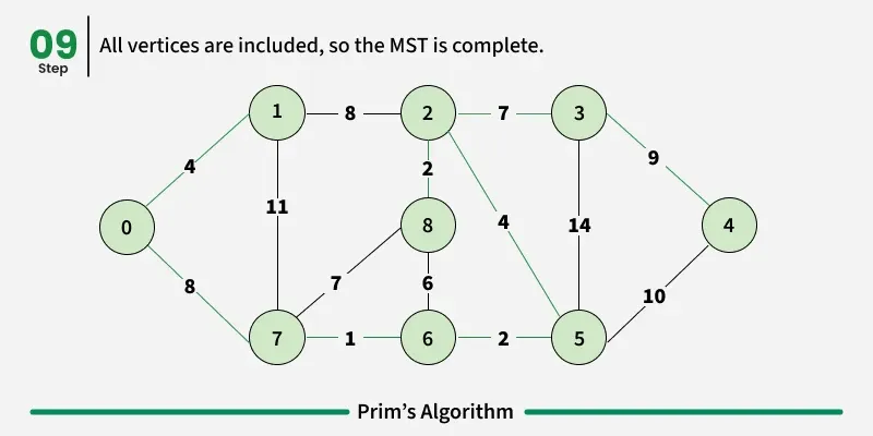
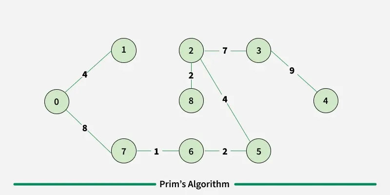
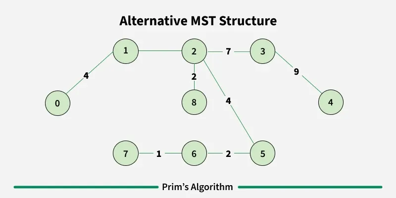
Working of the Prim’s Algorithm
1
2
3
4
5
6
7
8
9
10
11
12
13
14
15
16
17
18
19
20
21
22
23
24
25
26
27
28
29
30
31
32
33
34
35
36
37
38
39
40
41
42
43
44
45
46
47
48
49
50
51
52
53
54
55
56
57
58
59
60
61
62
63
64
65
66
67
68
69
70
71
72
73
74
75
76
77
78
79
80
81
82
83
84
import sys


class Graph():
    def __init__(self, vertices):
        self.V = vertices
        self.graph = [[0 for column in range(vertices)]
                      for row in range(vertices)]

    # A utility function to print
    # the constructed MST stored in parent[]
    def printMST(self, parent):
        print("Edge \tWeight")
        for i in range(1, self.V):
            print(parent[i], "-", i, "\t", self.graph[parent[i]][i])

    # A utility function to find the vertex with
    # minimum distance value, from the set of vertices
    # not yet included in shortest path tree
    def minKey(self, key, mstSet):

        # Initialize min value
        min = sys.maxsize

        for v in range(self.V):
            if key[v] < min and mstSet[v] == False:
                min = key[v]
                min_index = v

        return min_index

    # Function to construct and print MST for a graph
    # represented using adjacency matrix representation
    def primMST(self):

        # Key values used to pick minimum weight edge in cut
        key = [sys.maxsize] * self.V

        parent = [None] * self.V  # Array to store constructed MST

        # Make key 0 so that this vertex is picked as first vertex
        key[0] = 0

        mstSet = [False] * self.V

        parent[0] = -1  # First node is always the root of

        for cout in range(self.V):

            # Pick the minimum distance vertex from
            # the set of vertices not yet processed.
            # u is always equal to src in first iteration
            u = self.minKey(key, mstSet)

            # Put the minimum distance vertex in
            # the shortest path tree
            mstSet[u] = True

            # Update dist value of the adjacent vertices
            # of the picked vertex only if the current
            # distance is greater than new distance and
            # the vertex in not in the shortest path tree
            for v in range(self.V):

                # graph[u][v] is non zero only for adjacent vertices of m
                # mstSet[v] is false for vertices not yet included in MST
                # Update the key only if graph[u][v] is smaller than key[v]
                if self.graph[u][v] > 0 and mstSet[v] == False \
                and key[v] > self.graph[u][v]:
                    key[v] = self.graph[u][v]
                    parent[v] = u

        self.printMST(parent)


if __name__ == '__main__':
    g = Graph(5)
    g.graph = [[0, 2, 0, 6, 0],
               [2, 0, 3, 8, 5],
               [0, 3, 0, 0, 7],
               [6, 8, 0, 0, 9],
               [0, 5, 7, 9, 0]]

    g.primMST()
Output
1
2
3
4
5
Edge 	Weight
0 - 1 	2
1 - 2 	3
0 - 3 	6
1 - 4 	5
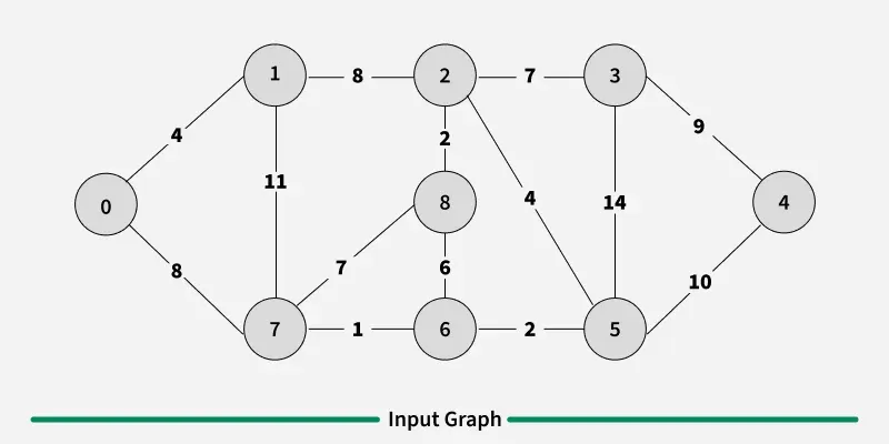
A minimum spanning tree (MST) or minimum weight spanning tree for a weighted, connected, and undirected graph is a spanning tree (no cycles and connects all vertices) that has minimum weight. The weight of a spanning tree is the sum of all edges in the tree.
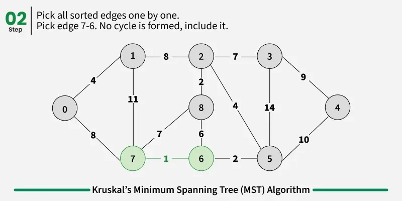
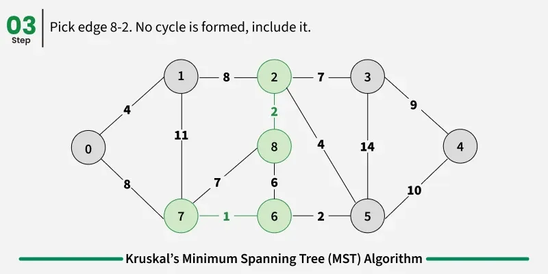
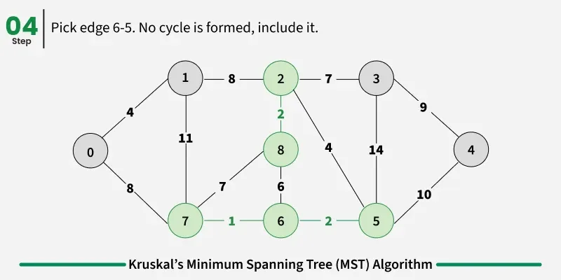
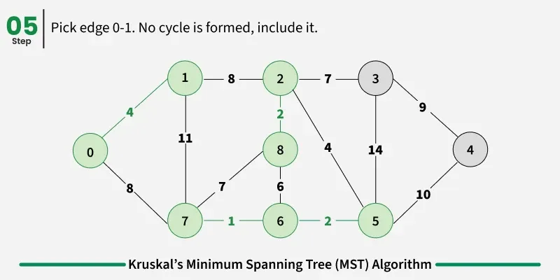
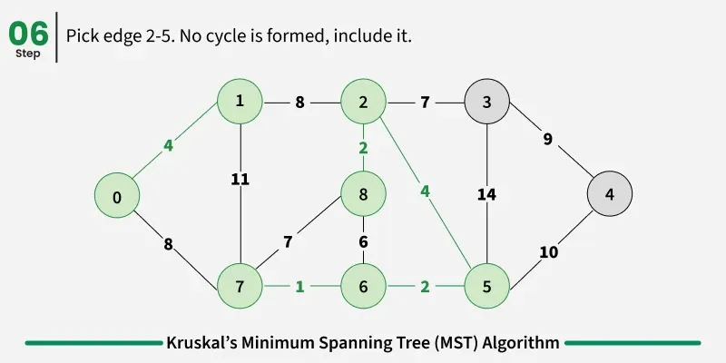
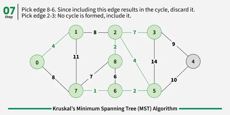
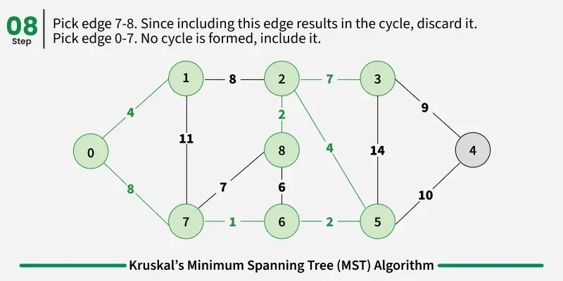
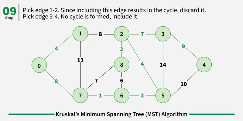
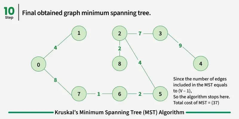
Below are the steps for finding MST using Kruskal’s algorithm:
It picks the minimum weighted edge at first and the maximum weighted edge at last. Thus we can say that it makes a locally optimal choice in each step in order to find the optimal solution. Hence this is a Greedy Algorithm.
Examples: The graph contains 9 vertices and 14 edges. So, the minimum spanning tree formed will be having (9 - 1) = 8 edges.

1
2
3
4
5
6
7
8
9
10
11
12
13
14
15
16
17
18
19
20
21
22
23
24
25
26
27
28
29
30
31
32
33
34
35
36
37
38
39
40
41
42
43
44
45
46
47
48
49
50
51
52
53
54
from functools import cmp_to_key

def comparator(a,b):
    return a[2] - b[2];

def kruskals_mst(V, edges):

    # Sort all edges
    edges = sorted(edges,key=cmp_to_key(comparator))

    # Traverse edges in sorted order
    dsu = DSU(V)
    cost = 0
    count = 0
    for x, y, w in edges:

        # Make sure that there is no cycle
        if dsu.find(x) != dsu.find(y):
            dsu.union(x, y)
            cost += w
            count += 1
            if count == V - 1:
                break
    return cost

# Disjoint set data structure
class DSU:
    def __init__(self, n):
        self.parent = list(range(n))
        self.rank = [1] * n

    def find(self, i):
        if self.parent[i] != i:
            self.parent[i] = self.find(self.parent[i])
        return self.parent[i]

    def union(self, x, y):
        s1 = self.find(x)
        s2 = self.find(y)
        if s1 != s2:
            if self.rank[s1] < self.rank[s2]:
                self.parent[s1] = s2
            elif self.rank[s1] > self.rank[s2]:
                self.parent[s2] = s1
            else:
                self.parent[s2] = s1
                self.rank[s1] += 1


if __name__ == '__main__':

    # An edge contains, weight, source and destination
    edges = [[0, 1, 10], [1, 3, 15], [2, 3, 4], [2, 0, 6], [0, 3, 5]]
    print(kruskals_mst(4, edges))
Output:
1
2
3
4
5
Following are the edges in the constructed MST
2 -- 3 == 4
0 -- 3 == 5
0 -- 1 == 10
Minimum Cost Spanning Tree: 19