Table of contents

Python’s Sequence Types

In Python, a sequence is a collection of elements stored in a specific order. Each element can be accessed by its index.

Python provides several array-based sequence types, meaning the elements are stored contiguously in memory, like an array.

The most important ones are:

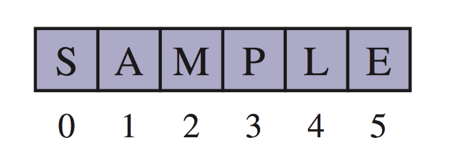
An array can store primitive elements, such as characters, giving us a compact array.

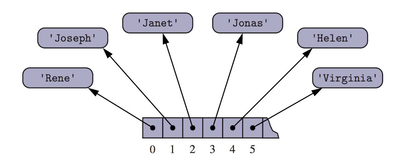
An array can also store references to objects.

Compact Arrays

1. What is a Compact Array?

A compact array stores elements in raw binary form, just like arrays in C.

Primary support for compact arrays is in a module named array. That module defines a class, also named array, providing compact storage for arrays of primitive data types.

This makes them:

• Much smaller in memory
• Faster for numerical data
• Restricted to one data type

Python implements this using:

1
from array import array

2. Creating an Array

The constructor for the array class requires a type code as a first parameter, which is a character that designates the type of data that will be stored in the array.

To create an array, you must specify:

• A type code
• An initial sequence of values

1
primes = array('i', [2, 3, 5, 7, 11, 13, 17, 19])

• ‘i’ = integer
• [10, 20, 30, 40] = initial data

Accessing Elements:

1
2
3
print(primes[0])     # 2
print(primes[1:3])   # array('i', [3, 5, 7])

You can also modify them:

1
2
primes[0] = 99
primes.append(50)

3. Type Codes

The type code tells Python what kind of data the array will store.

1
2
array('f', [1.2, 3.4, 5.6])
array('i', [1, 2, 3, 4])

4.Compact Arrays vs Lists

When to Use array Instead of list

• Use array when:
• All values have the same type
• You need high performance
• Memory usage matters

Use list when:

• Data types are mixed
• You need flexibility

Insertion in an Array

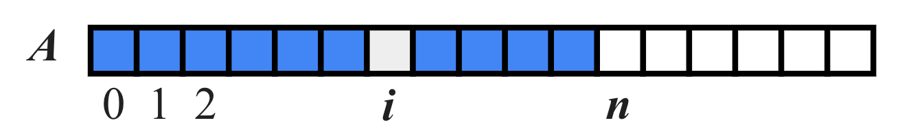
Consider an array with n elements:

1
A = [A0, A1, A2, ..., A(n−1)]

We perform an operation:

1
add(i, o)

• In an add(o) operation (without an index), we could always add at the end
• When the array is full, we replace the array with a larger one
• How large should the new array be?
  • Incremental strategy: increase the size by a constant c
  • Doubling strategy: double the size

1
2
3
4
5
6
7
Algorithm add(o)
	if t = S.length - 1 then A <- new array of size …
		for i = 0 to n-1 do
			 A[i] <- S[i]
		S <- A
	n <- n + 1
	S[n-1] <- o

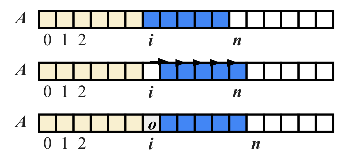
Which means insert object o at index i.

What Happens During Insertion?

To insert at position i, we must:

• Step 1: Make space for the new element
• Step 2: Shift all elements from index i to n−1 one position to the right

Notes:

• list.append() is fast
• list.insert(0, x) is slow

Why append() is fast

When you do:

1
lst.append(x)

Python:

1. Checks if there is free space at the end
2. If yes => stores x in the next empty slot
3. No elements need to move

So this is:

• O(1) (constant time, on average)

Example:

1
2
[10, 20, 30, _]  => append(40)
[10, 20, 30, 40]

Even when Python runs out of space, it:

• Allocates a larger block
• Copies everything once
• This happens rarely, so amortized time is still O(1).

Why insert(0, x) is slow

Now consider:

1
lst.insert(0, x)

You are inserting at the front.

Memory before:

1
[10, 20, 30, 40]

To put x at index 0, Python must:

1. Move 40 to index 4
2. Move 30 to index 3
3. Move 20 to index 2
4. Move 10 to index 1
5. Put x at index 0

Result:

1
[x, 10, 20, 30, 40]

Every element must be shifted one position to the right.

That is:

1
n moves for n elements => O(n)

Element Removal in an Array

Assume we have an array with n elements:

• A = [A0, A1, A2, …, A(n−1)]

We perform:

1
remove(i)

which means delete the element at index i.

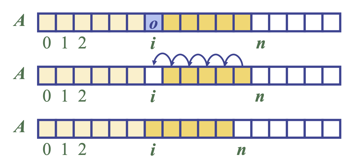
What Happens Internally?

When we remove A[i], we create a hole in the array:

1
2
3
1. Before: [A0, A1, A2, ..., A(n-1)]
2. remove(1) => remove A1
3. After hole: [A0,  _ , A2, A3, ..., A(n-1)]

To keep elements contiguous, we must shift everything after index i one position to the left:

1
A[i+1], A[i+2], ..., A[n−1]

Move to:

1
A[i], A[i+1], ..., A[n−2]

Final result:

1
[A0, A2, A3, ..., A(n-2)]

Performance of an Array-Based Dynamic List

In an array based implementation of a dynamic list:

• The space used by the data structure is O(n)
• Indexing the element at I takes O(1) time

1. Space Complexity

If the list stores n elements, it uses:

1
O(n) # space

Even though Python may allocate a little extra unused space, the memory grows linearly with the number of elements.

1. Indexing Time

Accessing an element:

1
A[i]  # Big-O: O(1)

This gives it very specific performance characteristics. Why?

Because the array stores elements in contiguous memory, so the address of A[i] is computed directly: address = base + i × element_size

1. Insertion and Removal

Full code python

1
2
3
4
5
6
7
8
9
10
11
12
13
14
15
16
17
18
19
20
21
22
23
24
25
26
27
28
29
30
31
32
33
34
35
36
37
38
39
40
41
42
43
44
45
46
47
48
49
50
51
52
53
54
55
56
57
58
59
60
61
62
63
64
65
66
67
import ctypes    # provides low-level arrays

class DynamicArray:
    """A dynamic array class akin to a simplified Python list."""

    def __init__(self):
        """Create an empty array."""
        self._n = 0                         # count actual elements
        self._capacity = 1                  # default array capacity
        self._A = self._make_array(self._capacity)

    def __len__(self):
        """Return number of elements stored in the array."""
        return self._n

    def __getitem__(self, k):
        """Return element at index k."""
        if not 0 <= k < self._n:
            raise IndexError('invalid index')
        return self._A[k]

    def append(self, obj):
        """Add object to end of the array."""
        if self._n == self._capacity:
            self._resize(2 * self._capacity)
        self._A[self._n] = obj
        self._n += 1

    def insert(self, i, x):
        """Insert element x at index i."""
        if not 0 <= i <= self._n:
            raise IndexError('invalid index')

        # resize if array is full
        if self._n == self._capacity:
            self._resize(2 * self._capacity)

        # shift elements to the right
        for k in range(self._n, i, -1):
            self._A[k] = self._A[k - 1]

        self._A[i] = x
        self._n += 1

    def remove(self, i):
        """Remove element at index i."""
        if not 0 <= i < self._n:
            raise IndexError('invalid index')

        # shift elements to the left
        for k in range(i, self._n - 1):
            self._A[k] = self._A[k + 1]

        self._A[self._n - 1] = None  # avoid loitering
        self._n -= 1

    def _resize(self, c):
        """Resize internal array to capacity c."""
        B = self._make_array(c)
        for k in range(self._n):
            B[k] = self._A[k]
        self._A = B
        self._capacity = c

    def _make_array(self, c):
        """Return new array with capacity c."""
        return (c * ctypes.py_object)()

Exercises

1. User Activity Log Management

An AI-enabled system needs to store user activity logs in chronological order.

Each log entry is represented as a tuple:

1
(user_id, action)

Example:

1
2
3
("u01", "login")
("u01", "view_page")
("u01", "logout")

1. Task 1 – Add a Log Entry

This task simulates recording a new user action in the system.

New log entries should always be added to the end of the log list, preserving chronological order.

Create a function as below:

1
def add_log(logs, user_id, action):

Input:

• logs: a DynamicArray object storing log entries
• user_id: string representing the user identifier
• action: string representing the user action

Output:

• No return value
• A new log (user_id, action) is appended to logs

Requirement

• Use the append() method of DynamicArray

1
2
3
4
5
6
7
8
9
10
11
12
13
def add_log(logs, user_id, action):
    """
    Task 1: Add a log entry to the end of the DynamicArray.

    Input:
        logs    : DynamicArray
        user_id : str
        action  : str

    Output:
        None
    """
    logs.append((user_id, action))

1. Task 2 – Insert a Priority Log

Some system events (e.g., security checks) must be logged before all other events.

This task inserts a high-priority log at the beginning of the log list.

Create a function as below:

1
def insert_priority_log(logs, user_id, action):

Input:

• logs: a DynamicArray object
• user_id: string
• action: string

Output:

• No return value
• A new log is inserted at index 0

Requirement

• Use insert(0, x)

1
2
3
4
5
6
7
8
9
10
11
12
13
def insert_priority_log(logs, user_id, action):
    """
    Task 2: Insert a high-priority log at the beginning of the DynamicArray.

    Input:
        logs    : DynamicArray
        user_id : str
        action  : str

    Output:
        None
    """
    logs.insert(0, (user_id, action))

1. Task 3 – Remove an Invalid Log

Sometimes a log entry is incorrect or corrupted and must be removed.

This task deletes a log entry at a specified position while maintaining the order of remaining logs.

Create a function as below:

1
def remove_log(logs, index):

Input:

• logs: a DynamicArray object
• index: integer index of the log to remove

Output:

• No return valueT
• The log at position index is removed

Requirement

• Use remove(index)

1
2
3
4
5
6
7
8
9
10
11
12
def remove_log(logs, index):
    """
    Task 3: Remove the log entry at the given index.

    Input:
        logs  : DynamicArray
        index : int

    Output:
        None
    """
    logs.remove(index)

1. Task 4 – Remove an Invalid Log

The system must be able to quickly retrieve a specific log entry for auditing or debugging purposes.

Create a function as below:

1
def get_log(logs, index):

Input:

• logs: a DynamicArray object
• index: integer

Output:

• Returns the log entry at position index
• Type: tuple (user_id, action)

Requirement

• Use array indexing (logs[index])

1
2
3
4
5
6
7
8
9
10
11
12
def get_log(logs, index):
    """
    Task 4: Retrieve the log entry at the given index.

    Input:
        logs  : DynamicArray
        index : int

    Output:
        tuple (user_id, action)
    """
    return logs[index]

1. Using:

1
2
3
4
5
6
7
8
9
10
11
12
13
14
15
16
17
18
from dynamicArray import DynamicArray

# ... task 1
# ... task 2
# ... task 3
# ... task 4

logs = DynamicArray()

add_log(logs, "u01", "login")
add_log(logs, "u01", "view_page")
insert_priority_log(logs, "admin", "system_check")

print(get_log(logs, 0))
# ('admin', 'system_check')

remove_log(logs, 1)

Queue

A Queue ADT stores arbitrary objects and follows the First-In, First-Out (FIFO) principle.

The first element inserted into the queue is the first one removed.

Queue Discipline (FIFO)

• Insertion happens at the rear of the queue
• Removal happens at the front of the queue

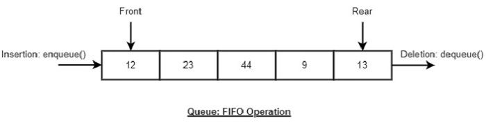
Main queue operations:

• enqueue(object): inserts an element at the end of the queue
• object dequeue(): removes and returns the element at the front of the queue

Auxiliary queue operations:

• object first(): returns the element at the front without removing it
• integer len(): returns the number of elements stored
• boolean is_empty(): indicates whether no elements are stored

Exceptions: Attempting the execution of dequeue or front on an empty queue throws an EmptyQueueException

Time Complexity (Array-Based Queue)

Array-Based Queue Implementation

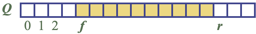
A queue can be efficiently implemented using an array of fixed size N in a circular fashion.

Instead of shifting elements, the array is treated as circular, wrapping around when the end is reached.

Two integer variables are used to track the queue:

• f: index of the front element
• r: index immediately past the rear element

Important rule

• Array location r is always kept empty
• This helps distinguish between full and empty states

1
2
Array indices: 0  1  2  3  4  ...  N-1
Queue wraps around using modulo arithmetic

Size Operation

1
2
Algorithm size()
	return (N - f + r) mod N

Explanation:

• Computes the number of elements stored
• Works correctly even when indices wrap around

isEmpty Operation

1
2
Algorithm isEmpty()
    return (f = r)

Explanation:

• When f == r, the queue contains no elements

Enqueue Operation (Full Queue Case)

The enqueue operation inserts an element at position r

After insertion: r <- (r + 1) mod N

1
2
3
4
5
6
Algorithm enqueue(o)
	if size() = N <- 1 then
		throw FullQueueException
	 else  
		Q[r] <- o
		r <- (r + 1) mod N

In this case:

• enqueue throws an exception
• The specific exception type is implementation-dependent

Queue ADT function:

Direct applications

• Waiting lists, bureaucracy
• Access to shared resources (e.g., printer)
• Multiprogramming

Indirect applications

• Auxiliary data structure for algorithms
• Component of other data structures

Array-based Queue

• Use an array of size N in a circular fashion
• Two variables keep track of the front and rear
  • f index of the front element
  • r index immediately past the rear element Array location r is kept empty

Queue Operations

• We use the modulo operator (remainder of division)

1
2
3
4
5
Algorithm size()
	return (N - f + r) mod N

Algorithm isEmpty()
	return (f = r)

• Operation enqueue throws an exception if the array is full
• This exception is implementation-dependent

1
2
Operation enqueue throws an exception if the array is full
This exception is implementation-dependent

Stack

Abstract Data Type (ADT)

An Abstract Data Type (ADT) is an abstraction of a data structure. It defines what operations are supported and how the data behaves, without specifying how the data is implemented.

An ADT specifies:

• Data stored
• Operations on the data
• Error conditions associated with operations

Example: ADT for a Stock Trading System

Data Stored: Buy and sell orders

Supported Operations

1
2
3
order buy(stock, shares, price)
order sell(stock, shares, price)
void cancel(order)

Error Conditions

• Buying or selling a nonexistent stock
• Canceling a nonexistent order

Basic Terminologies of Queue

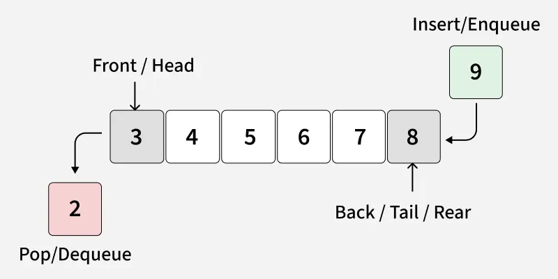
Front: Position of the entry in a queue ready to be served, that is, the first entry that will be removed from the queue, is called the front of the queue. It is also referred as the head of the queue.

Rear: Position of the last entry in the queue, that is, the one most recently added, is called the rear of the queue. It is also referred as the tail of the queue.

Size: Size refers to the current number of elements in the queue.

Capacity: Capacity refers to the maximum number of elements the queue can hold.

Hash Table

A Hash table is defined as a data structure used to insert, look up, and remove key-value pairs quickly. It operates on the hashing concept, where each key is translated by a hash function into a distinct index in an array. The index functions as a storage location for the matching value. In simple words, it maps the keys with the value.

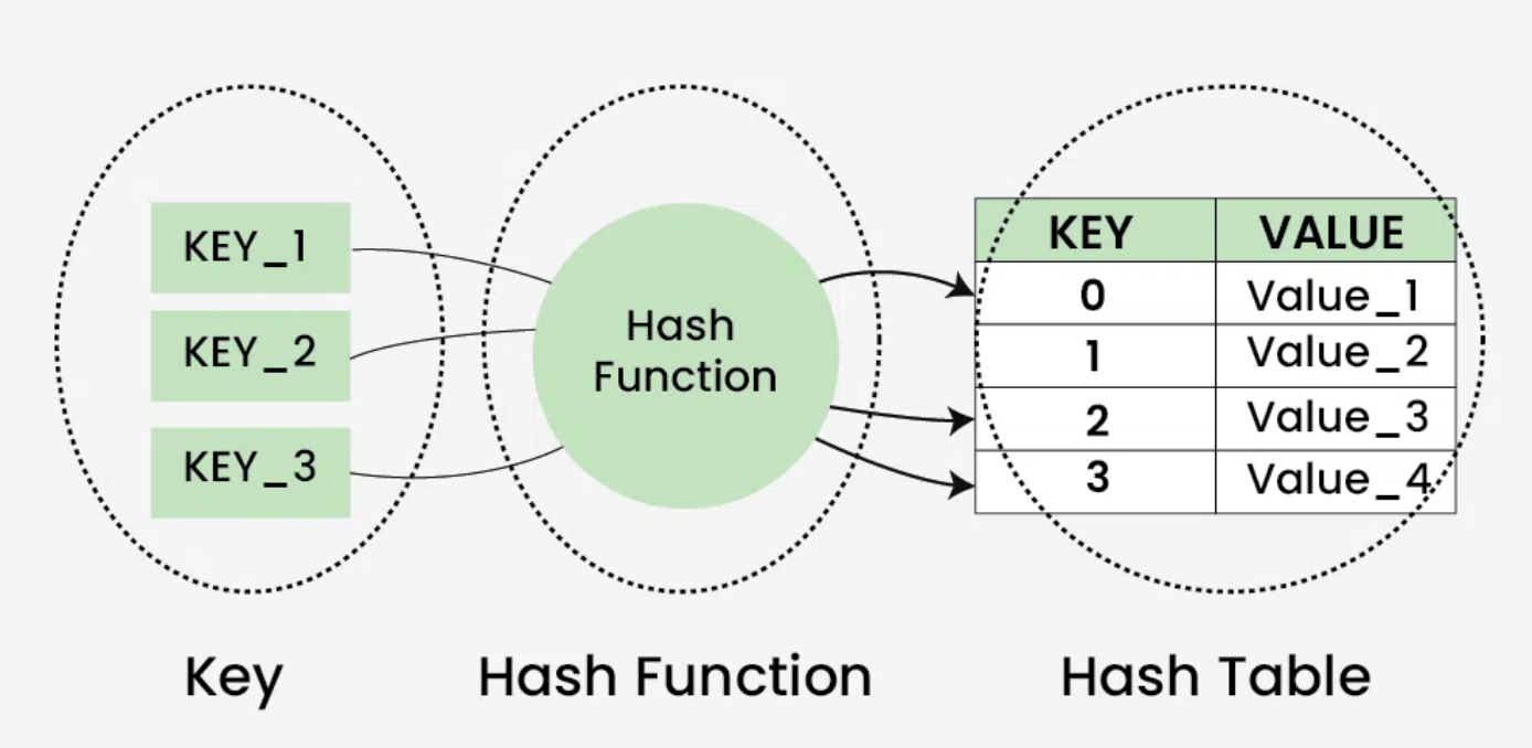
Input: Data goes into the hashing algorithm. Hash Function: Math magic creates a fixed-size hash. Output: Hash becomes the index for data storage or retrieval.

Hash function

There are many hash functions that use numeric or alphanumeric keys. This article focuses on discussing different hash functions:

• Division Method.
• Mid Square Method.
• Folding Method.
• Multiplication Method

1. Division Method

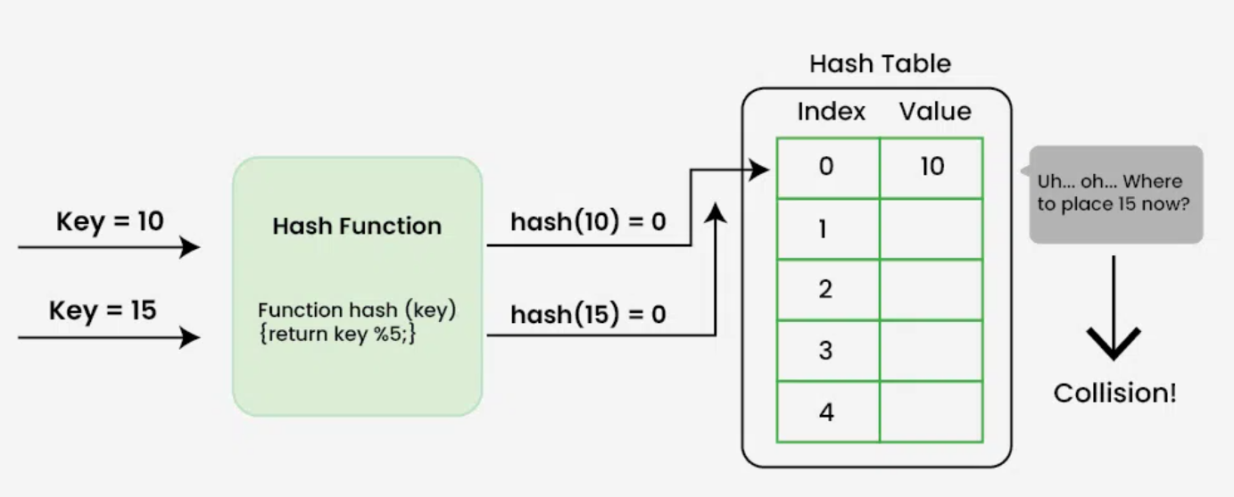
This is the most simple and easiest method to generate a hash value. The hash function divides the value k by M and then uses the remainder obtained.

1
**h(K) = k mod M**

Here,

• k is the key value, and
• M is the size of the hash table.

2. Mid Square Method

The mid-square method is a very good hashing method. It involves two steps to compute the hash value-

• Square the value of the key k i.e. k2
• Extract the middle r digits as the hash value.

1
h(k) = h(k x k)

Here, k is the key value.

3. Folding Method

This method involves two steps:

Divide the key-value k into a number of parts i.e. k1, k2, k3,….,kn, where each part has the same number of digits except for the last part that can have lesser digits than the other parts. Add the individual parts. The hash value is obtained by ignoring the last carry if any.

1
2
3
k = k1, k2, k3, k4, ….., kn
s = k1+ k2 + k3 + k4 +….+ kn
h(K)= s

Here, s is obtained by adding the parts of the key k

Example:

1
2
3
4
5
6
k = 12345
k1 = 12, k2 = 34, k3 = 5
s = k1 + k2 + k3
  = 12 + 34 + 5
  = 51 
h(K) = 51

4. Multiplication Method

This method involves the following steps:

1. Choose a constant value A such that 0 < A < 1.
2. Multiply the key value with A.
3. Extract the fractional part of kA.
4. Multiply the result of the above step by the size of the hash table i.e. M.
5. The resulting hash value is obtained by taking the floor of the result obtained in step 4.

1
h(K) = floor (M (kA mod 1))

Here,

• M is the size of the hash table.
• k is the key value.
• A is a constant value.

Example:

1
2
3
4
5
6
7
8
k = 12345
A = 0.357840
M = 100

h(12345) = floor[ 100 (12345*0.357840 mod 1)]
               = floor[ 100 (4417.5348 mod 1) ]
               = floor[ 100 (0.5348) ]
               = floor[ 53 ]

Collision resolution techniques:

• Open Addressing
• Separate Chaining

1. Open Addressing

2. Separate Chaining

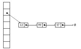
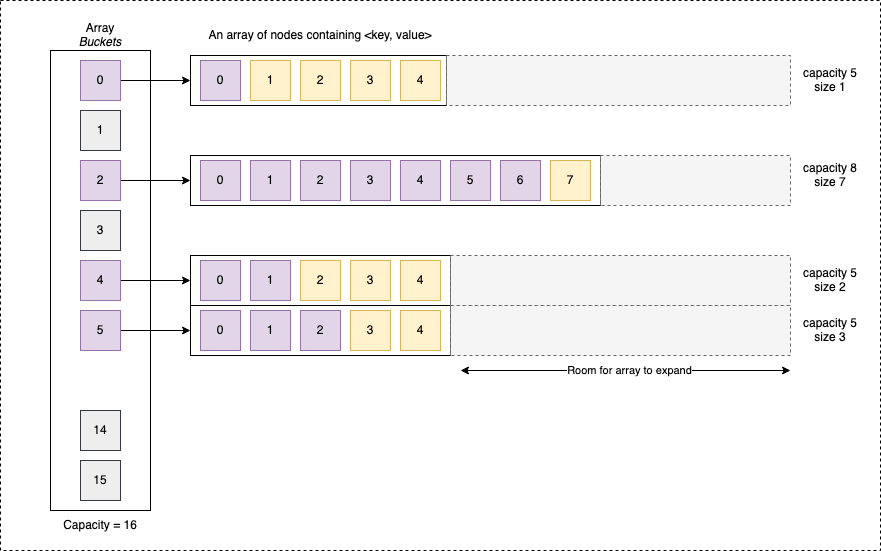
The idea behind Separate Chaining is to make each cell of the hash table point to a linked list of records that have the same hash function value. Chaining is simple but requires additional memory outside the table.

Example: We have given a hash function and we have to insert some elements in the hash table using a separate chaining method for collision resolution technique.

Below are different options to create chains.

• The advantage of linked list implementation is insert is O(1) in the worst case.
• The advantage of array is cache friendliness, but the insert operation can be O(1) in cases when we have to resize the array.
• The advantage of Self Balancing BST is the worst case is bounded by O(Log (len)) for all operations

Priority Queue

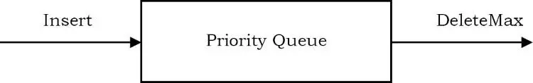
A priority queue is a special type of queue in which each element is associated with a priority value. And, elements are served on the basis of their priority. That is, higher priority elements are served first.

However, if elements with the same priority occur, they are served according to their order in the queue.

Assigning Priority Value

Generally, the value of the element itself is considered for assigning the priority. For example,

The element with the highest value is considered the highest priority element. However, in other cases, we can assume the element with the lowest value as the highest priority element.

We can also set priorities according to our needs.

Difference between Priority Queue and Normal Queue

Queue: The first-in-first-out rule is implemented whereas,

Priority queue, the values are removed on the basis of priority. The element with the highest priority is removed first.

Main Operations on Priority Queues

A priority queue is a container of elements, where each element is associated with a key.

• Insert (key, data): Add an element with its key into the priority queue.
• DeleteMin / DeleteMax: Remove and return the element with the smallest/largest key.
• GetMinimum / GetMaximum: Return the element with the smallest/largest key without removing it.

Auxiliary Operations on Priority Queues

• kth Smallest / kth Largest: Return the k-th smallest/largest key in the priority queue.
• Size: Return the number of elements in the priority queue.
• Heap Sort: Sort the elements in the priority queue based on their priority (key).

A comparative analysis of different implementations of priority queue is given below.

Implements Priority Queue:

Priority Queue implement by Linked List

1
2
3
4
5
6
7
8
9
10
11
12
13
14
15
16
17
18
19
20
21
22
23
24
25
26
27
28
29
30
31
32
33
34
35
36
37
38
39
class PriorityQueueLinkedList:
    class Node:
        def __init__(self, key, data):
            self.key = key
            self.data = data
            self.next = None
    
    def __init__(self):
        self.root = None

    def isEmpty(self):
        return self.root is None

    def enqueue(self, key, data):
        newNode = self.Node(key, data)

        if self.isEmpty() or key < self.root.key:
            newNode.next = self.root
            self.root = newNode
        else:
            current = self.root
            while current.next and current.next.key <= key:
                current = current.next
            
            newNode.next = current.next
            current.next = newNode

    def dequeue(self):
        if self.isEmpty():
            raise IndexError("Priority Queue is empty")

        node = self.root
        self.root = self.root.next
        return (node.key, node.data)

    def peek(self):
        if self.isEmpty():
            raise IndexError("Priority Queue is empty")
        return (self.root.key, self.root.data)

Priority Queue implement by Binary Heap

1
2
3
4
5
6
7
8
9
10
11
12
13
14
15
16
17
18
19
20
21
22
23
24
25
26
27
28
29
30
31
32
33
34
35
36
37
38
39
40
41
42
43
44
45
46
47
48
49
50
51
52
53
54
class PriorityQueueHeap:
    def __init__(self):
        self.heap = []

    def isEmpty(self):
        return len(self.heap) == 0

    def enqueue(self, key, data):
        self.heap.append((key, data))
        self._heapify_up(len(self.heap) - 1)

    def _heapify_up(self, i):
        parent = (i - 1) // 2
        while i > 0 and self.heap[i][0] < self.heap[parent][0]:
            self.heap[i], self.heap[parent] = self.heap[parent], self.heap[i]
            i = parent
            parent = (i - 1) // 2

    def dequeue(self):
        if self.isEmpty():
            raise IndexError("Priority Queue is empty")

        root = self.heap[0]
        last = self.heap.pop()

        if not self.isEmpty():
            self.heap[0] = last
            self._heapify_down(0)

        return root

    def _heapify_down(self, i):
        size = len(self.heap)

        while True:
            smallest = i
            left = 2 * i + 1
            right = 2 * i + 2

            if left < size and self.heap[left][0] < self.heap[smallest][0]:
                smallest = left
            if right < size and self.heap[right][0] < self.heap[smallest][0]:
                smallest = right

            if smallest != i:
                self.heap[i], self.heap[smallest] = self.heap[smallest], self.heap[i]
                i = smallest
            else:
                break

    def peek(self):
        if self.isEmpty():
            raise IndexError("Priority Queue is empty")
        return self.heap[0]

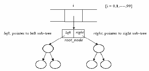
Priority Queue (Binary Search Tree)

1
2
3
4
5
6
7
8
9
10
11
12
13
14
15
16
17
18
19
20
21
22
23
24
25
26
27
28
29
30
31
32
33
34
35
36
37
38
39
40
41
42
43
44
45
46
47
48
49
50
class PriorityQueueBST:
    class Node:
        def __init__(self, key, data):
            self.key = key
            self.data = data
            self.left = None
            self.right = None

    def __init__(self):
        self.root = None

    def isEmpty(self):
        return self.root is None

    def enqueue(self, key, data):
        self.root = self._insert(self.root, key, data)

    def _insert(self, node, key, data):
        if node is None:
            return self.Node(key, data)

        if key < node.key:
            node.left = self._insert(node.left, key, data)
        else:
            node.right = self._insert(node.right, key, data)

        return node

    def dequeue(self):
        if self.isEmpty():
            raise IndexError("Priority Queue is empty")

        self.root, minNode = self._deleteMin(self.root)
        return (minNode.key, minNode.data)

    def _deleteMin(self, node):
        if node.left is None:
            return node.right, node

        node.left, minNode = self._deleteMin(node.left)
        return node, minNode

    def peek(self):
        if self.isEmpty():
            raise IndexError("Priority Queue is empty")

        current = self.root
        while current.left:
            current = current.left
        return (current.key, current.data)