Simple NN graph:
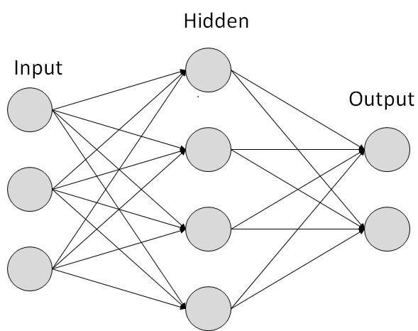
Deep NN consists of more hidden layers (Deeper layers)
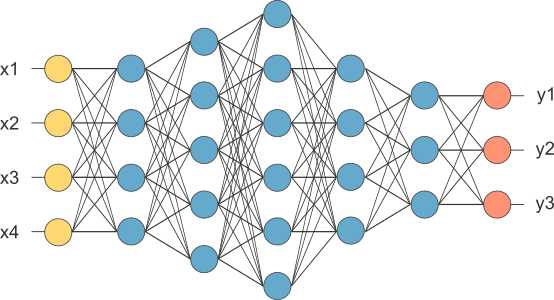
Table of contents
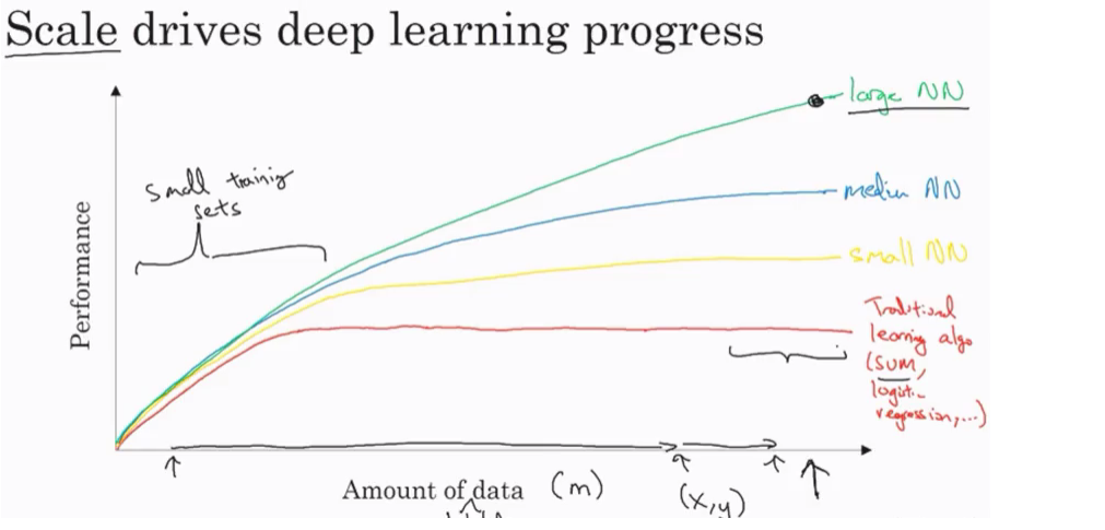
Be able to explain the major trends driving the rise of Machine Learning, and understand where and how it is applied today.
Simple NN graph:
Deep NN consists of more hidden layers (Deeper layers)
Learn to set up a machine learning problem with a neural network mindset. Learn to use vectorization to speed up your models.
M is the number of training vectorsNx is the size of the input vectorNy is the size of the output vectorX(1) is the first input vectorY(1) is the first output vectorX = [x(1) x(2).. x(M)]Y = (y(1) y(2).. y(M))y = wx + by = w(transpose)x + by = sigmoid(w(transpose)x + b)y = sigmoid(w(transpose)x)
b is w0 of w and we add x0 = 1. but we won’t use this notation in the course (Andrew said that the first notation is better).Y has to be between 0 and 1.w is a vector of Nx and b is a real numberL(y',y) = 1/2 (y' - y)^2
L(y',y) = - (y*log(y') + (1-y)*log(1-y'))y = 1 ==> L(y',1) = -log(y') ==> we want y' to be the largest ==> y’ biggest value is 1y = 0 ==> L(y',0) = -log(1-y') ==> we want 1-y' to be the largest ==> y' to be smaller as possible because it can only has 1 value.J(w,b) = (1/m) * Sum(L(y'[i],y[i]))w and b that minimize the cost function.w and b to 0,0 or initialize them to a random value in the convex function and then try to improve the values the reach minimum value.w = w - alpha * dw
where alpha is the learning rate and dw is the derivative of w (Change to w)
The derivative is also the slope of wLooks like greedy algorithms. the derivative give us the direction to improve our parameters.
w = w - alpha * d(J(w,b) / dw) (how much the function slopes in the w direction)b = b - alpha * d(J(w,b) / db) (how much the function slopes in the d direction)f(a) = 3a d(f(a))/d(a) = 3a = 2 then f(a) = 6a = 2.001 then f(a) = 6.003 means that we multiplied the derivative (Slope) to the moved area and added it to the last result.f(a) = a^2 ==> d(f(a))/d(a) = 2a
a = 2 ==> f(a) = 4a = 2.0001 ==> f(a) = 4.0004 approx.f(a) = a^3 ==> d(f(a))/d(a) = 3a^2f(a) = log(a) ==> d(f(a))/d(a) = 1/a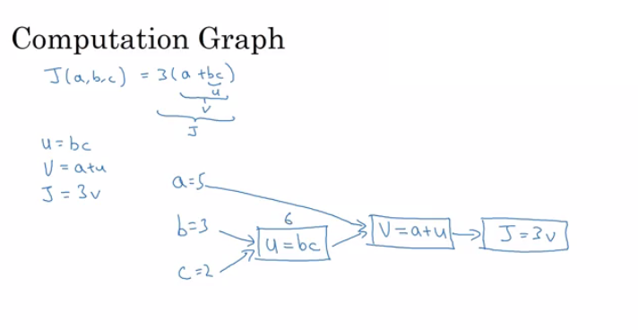
x -> y -> z (x effect y and y effects z)
Then d(z)/d(x) = d(z)/d(y) * d(y)/d(x)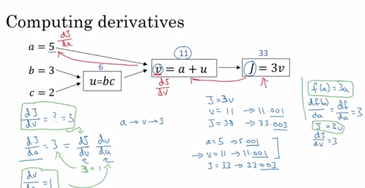
dvar means the derivatives of a final output variable with respect to various intermediate quantities.x1 and x2.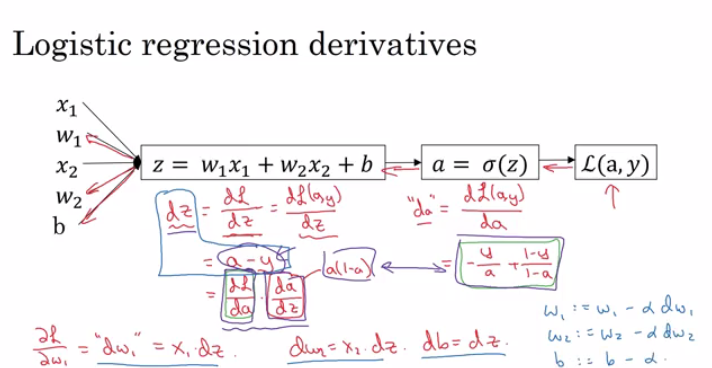
Lets say we have these variables:
1
2
3
4
5
6
7
	X1                  Feature
	X2                  Feature
	W1                  Weight of the first feature.
	W2                  Weight of the second feature.
	B                   Logistic Regression parameter.
	M                   Number of training examples
	Y(i)                Expected output of i
So we have:
Then from right to left we will calculate derivations compared to the result:
1
2
3
4
5
	d(a)  = d(l)/d(a) = -(y/a) + ((1-y)/(1-a))
	d(z)  = d(l)/d(z) = a - y
	d(W1) = X1 * d(z)
	d(W2) = X2 * d(z)
	d(B)  = d(z)
From the above we can conclude the logistic regression pseudo code:
1
2
3
4
5
6
7
8
9
10
11
12
13
14
15
16
17
18
19
20
21
22
	J = 0; dw1 = 0; dw2 =0; db = 0;                 # Devs.
	w1 = 0; w2 = 0; b=0;							# Weights
	for i = 1 to m
		# Forward pass
		z(i) = W1*x1(i) + W2*x2(i) + b
		a(i) = Sigmoid(z(i))
		J += (Y(i)*log(a(i)) + (1-Y(i))*log(1-a(i)))

		# Backward pass
		dz(i) = a(i) - Y(i)
		dw1 += dz(i) * x1(i)
		dw2 += dz(i) * x2(i)
		db  += dz(i)
	J /= m
	dw1/= m
	dw2/= m
	db/= m

	# Gradient descent
	w1 = w1 - alpha * dw1
	w2 = w2 - alpha * dw2
	b = b - alpha * db
The above code should run for some iterations to minimize error.
So there will be two inner loops to implement the logistic regression.
Vectorization is so important on deep learning to reduce loops. In the last code we can make the whole loop in one step using vectorization!
X and its [Nx, m] and a matrix Y and its [Ny, m].We will then compute at instance [z1,z2...zm] = W' * X + [b,b,...b]. This can be written in python as:
Vectorizing Logistic Regression’s Gradient Output:
dz = A - Y # Vectorization, dz shape is (1, m) dw = np.dot(X, dz.T) / m # Vectorization, dw shape is (Nx, 1) db = dz.sum() / m # Vectorization, dz shape is (1, 1)obj.sum(axis = 0) sums the columns while obj.sum(axis = 1) sums the rows.obj.reshape(1,4) changes the shape of the matrix by broadcasting the values.(m,) and the transpose operation won’t work. You have to reshape it to (m, 1)assert(a.shape == (5,1)) to check if your matrix shape is the required one.jupyter-notebook It should be installed to work.To Compute the derivative of Sigmoid:
1
2
	s = sigmoid(x)
	ds = s * (1 - s)       # derivative  using calculus
To make an image of (width,height,depth) be a vector, use this:
1
v = image.reshape(image.shape[0]*image.shape[1]*image.shape[2],1)  #reshapes the image.
Learn to build a neural network with one hidden layer, using forward propagation and backpropagation.
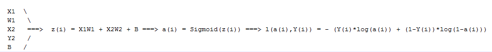
In logistic regression we had:
1
2
3
X1  \
X2   ==>  z = XW + B ==> a = Sigmoid(z) ==> l(a,Y)
X3  /
In neural networks with one layer we will have:
1
2
3
X1  \
X2   =>  z1 = XW1 + B1 => a1 = Sigmoid(z1) => z2 = a1W2 + B2 => a2 = Sigmoid(z2) => l(a2,Y)
X3  /
X is the input vector (X1, X2, X3), and Y is the output variable (1x1)a0 = x (the input layer)a1 will represent the activation of the hidden neurons.a2 will represent the output layer.
noOfHiddenNeurons = 4Nx = 3W1 is the matrix of the first hidden layer, it has a shape of (noOfHiddenNeurons,nx)b1 is the matrix of the first hidden layer, it has a shape of (noOfHiddenNeurons,1)z1 is the result of the equation z1 = W1*X + b, it has a shape of (noOfHiddenNeurons,1)a1 is the result of the equation a1 = sigmoid(z1), it has a shape of (noOfHiddenNeurons,1)W2 is the matrix of the second hidden layer, it has a shape of (1,noOfHiddenNeurons)b2 is the matrix of the second hidden layer, it has a shape of (1,1)z2 is the result of the equation z2 = W2*a1 + b, it has a shape of (1,1)a2 is the result of the equation a2 = sigmoid(z2), it has a shape of (1,1)Pseudo code for forward propagation for the 2 layers NN:
1
2
3
4
5
for i = 1 to m
  z[1, i] = W1*x[i] + b1      # shape of z[1, i] is (noOfHiddenNeurons,1)
  a[1, i] = sigmoid(z[1, i])  # shape of a[1, i] is (noOfHiddenNeurons,1)
  z[2, i] = W2*a[1, i] + b2   # shape of z[2, i] is (1,1)
  a[2, i] = sigmoid(z[2, i])  # shape of a[2, i] is (1,1)
Lets say we have X on shape (Nx,m). So the new pseudo code:
1
2
3
4
Z1 = W1X + b1     # shape of Z1 (noOfHiddenNeurons,m)
A1 = sigmoid(Z1)  # shape of A1 (noOfHiddenNeurons,m)
Z2 = W2A1 + b2    # shape of Z2 is (1,m)
A2 = sigmoid(Z2)  # shape of A2 is (1,m)
In the last example we can call X = A0. So the previous step can be rewritten as:
1
2
3
4
Z1 = W1A0 + b1    # shape of Z1 (noOfHiddenNeurons,m)
A1 = sigmoid(Z1)  # shape of A1 (noOfHiddenNeurons,m)
Z2 = W2A1 + b2    # shape of Z2 is (1,m)
A2 = sigmoid(Z2)  # shape of A2 is (1,m)
A = 1 / (1 + np.exp(-z)) # Where z is the input matrixIn NumPy we can implement Tanh using one of these methods:
A = (np.exp(z) - np.exp(-z)) / (np.exp(z) + np.exp(-z)) # Where z is the input matrix
Or
A = np.tanh(z) # Where z is the input matrix
RELU = max(0,z) # so if z is negative the slope is 0 and if z is positive the slope remains linear.Leaky_RELU = max(0.01z,z) #the 0.01 can be a parameter for your algorithm.Derivation of Sigmoid activation function:
1
2
3
g(z)  = 1 / (1 + np.exp(-z))
g'(z) = (1 / (1 + np.exp(-z))) * (1 - (1 / (1 + np.exp(-z))))
g'(z) = g(z) * (1 - g(z))
Derivation of Tanh activation function:
1
2
g(z)  = (e^z - e^-z) / (e^z + e^-z)
g'(z) = 1 - np.tanh(z)^2 = 1 - g(z)^2
Derivation of RELU activation function:
1
2
3
g(z)  = np.maximum(0,z)
g'(z) = { 0  if z < 0
          1  if z >= 0  }
Derivation of leaky RELU activation function:
1
2
3
g(z)  = np.maximum(0.01 * z, z)
g'(z) = { 0.01  if z < 0
          1     if z >= 0   }
n[0] = Nxn[1] = NoOfHiddenNeuronsn[2] = NoOfOutputNeurons = 1W1 shape is (n[1],n[0])b1 shape is (n[1],1)W2 shape is (n[2],n[1])b2 shape is (n[2],1)I = I(W1, b1, W2, b2) = (1/m) * Sum(L(Y,A2))Then Gradient descent:
1
2
3
4
5
6
7
Repeat:
		Compute predictions (y'[i], i = 0,...m)
		Get derivatives: dW1, db1, dW2, db2
		Update: W1 = W1 - LearningRate * dW1
				b1 = b1 - LearningRate * db1
				W2 = W2 - LearningRate * dW2
				b2 = b2 - LearningRate * db2
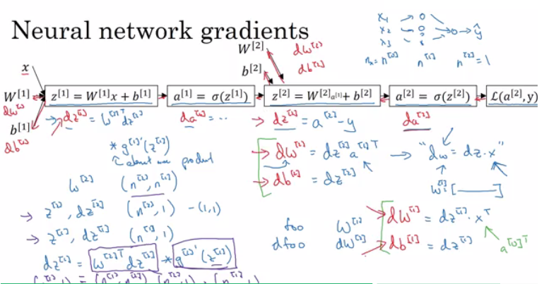
Forward propagation:
1
2
3
4
Z1 = W1A0 + b1    # A0 is X
A1 = g1(Z1)
Z2 = W2A1 + b2
A2 = Sigmoid(Z2)      # Sigmoid because the output is between 0 and 1
1
2
3
4
5
6
7
dZ2 = A2 - Y      # derivative of cost function we used * derivative of the sigmoid function
dW2 = (dZ2 * A1.T) / m
db2 = Sum(dZ2) / m
dZ1 = (W2.T * dZ2) * g'1(Z1)  # element wise product (*)
dW1 = (dZ1 * A0.T) / m   # A0 = X
db1 = Sum(dZ1) / m
# Hint there are transposes with multiplication because to keep dimensions correct
In logistic regression it wasn’t important to initialize the weights randomly, while in NN we have to initialize them randomly.
To solve this we initialize the W’s with a small random numbers:
1
2
W1 = np.random.randn((2,2)) * 0.01    # 0.01 to make it small enough
b1 = np.zeros((2,1))                  # its ok to have b as zero, it won't get us to the symmetry breaking problem
We need small values because in sigmoid (or tanh), for example, if the weight is too large you are more likely to end up even at the very start of training with very large values of Z. Which causes your tanh or your sigmoid activation function to be saturated, thus slowing down learning. If you don’t have any sigmoid or tanh activation functions throughout your neural network, this is less of an issue.
Understand the key computations underlying deep learning, use them to build and train deep neural networks, and apply it to computer vision.
L to denote the number of layers in a NN.n[l] is the number of neurons in a specific layer l.n[0] denotes the number of neurons input layer. n[L] denotes the number of neurons in output layer.g[l] is the activation function.a[l] = g[l](z[l])w[l] weights is used for z[l]x = a[0], a[l] = y'n of shape (1, NoOfLayers+1)g of shape (1, NoOfLayers)w based on the number of neurons on the previous and the current layer.b based on the number of neurons on the current layer.Forward propagation general rule for one input:
1
2
z[l] = W[l]a[l-1] + b[l]
a[l] = g[l](a[l])
Forward propagation general rule for m inputs:
1
2
Z[l] = W[l]A[l-1] + B[l]
A[l] = g[l](A[l])
W is (n[l],n[l-1]) . Can be thought by right to left.b is (n[l],1)dw has the same shape as W, while db is the same shape as bZ[l], A[l], dZ[l], and dA[l] is (n[l],m)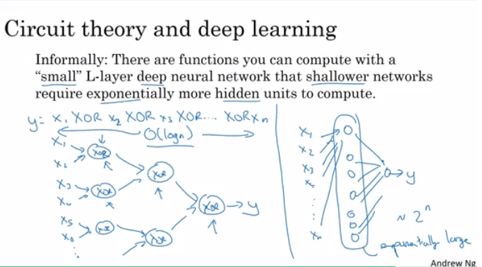
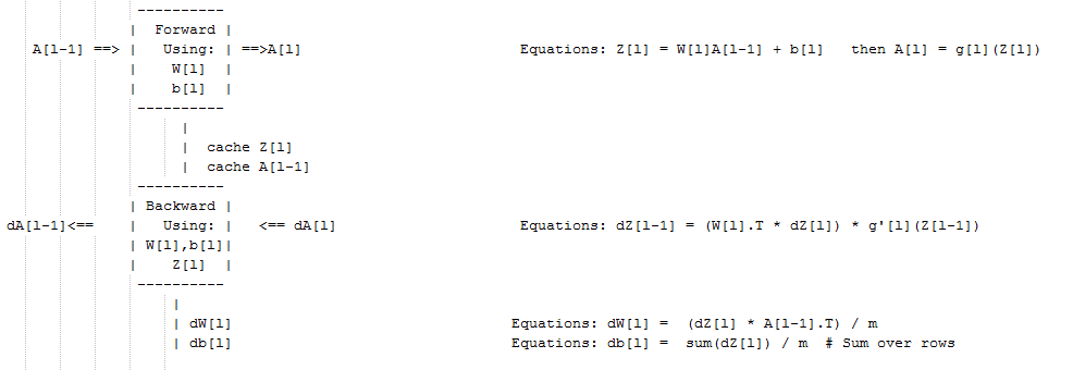
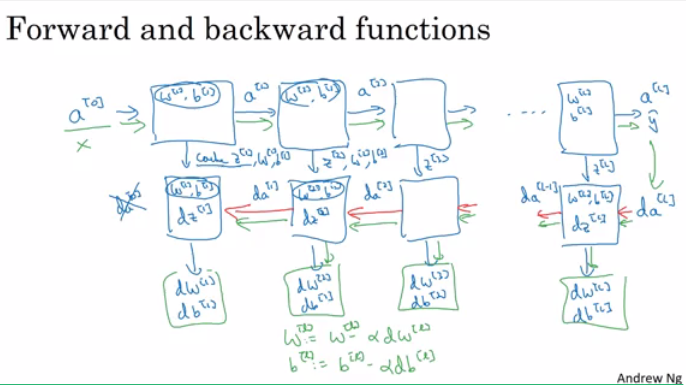
Pseudo code for forward propagation for layer l:
1
2
3
4
Input  A[l-1]
Z[l] = W[l]A[l-1] + b[l]
A[l] = g[l](Z[l])
Output A[l], cache(Z[l])
Pseudo code for back propagation for layer l:
1
2
3
4
5
6
Input da[l], Caches
dZ[l] = dA[l] * g'[l](Z[l])
dW[l] = (dZ[l]A[l-1].T) / m
db[l] = sum(dZ[l])/m                # Dont forget axis=1, keepdims=True
dA[l-1] = w[l].T * dZ[l]            # The multiplication here are a dot product.
Output dA[l-1], dW[l], db[l]
If we have used our loss function then:
1
dA[L] = (-(y/a) + ((1-y)/(1-a)))
W and bL.n.