Data cleaning is a step in machine learning (ML) which involves identifying and removing any missing, duplicate or irrelevant data.
Data Cleansing is a data preprocessing step that focuses on:
The goal is to produce a dataset that is:
Data cleansing is a critical part of Data Preparation and is performed before:
The process begins by identifying issues like missing values, duplicates and outliers. Performing data cleaning involves a systematic process to identify and remove errors in a dataset. The following steps are essential to perform data cleaning:
Import all the necessary libraries i.e pandas and numpy.
1
2
3
4
5
6
import pandas as pd
import numpy as np
df = pd.read_csv('Titanic-Dataset.csv')
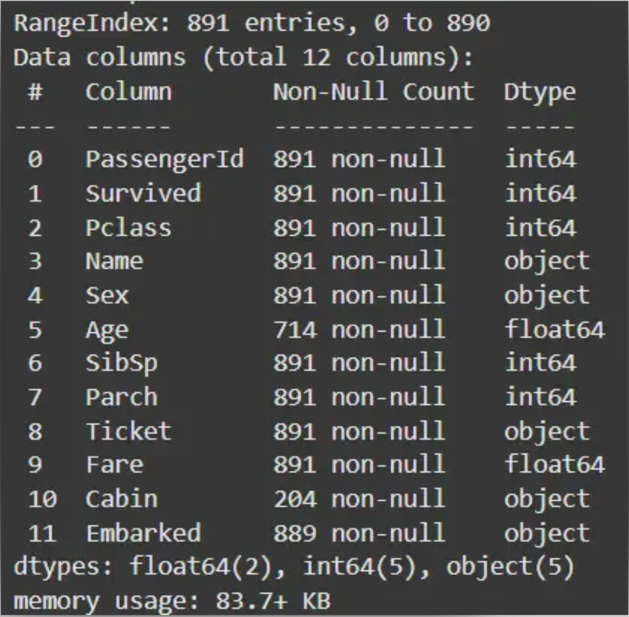
df.info()
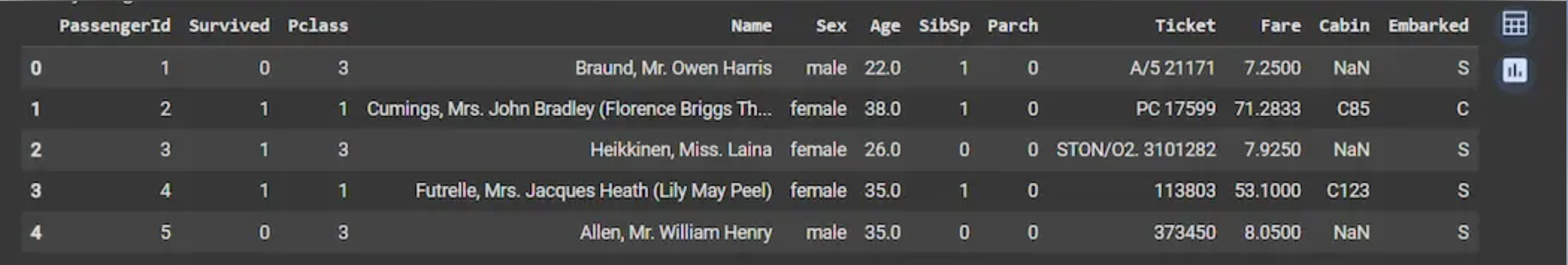
df.head()
Output:
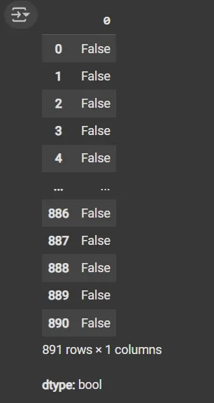
df.duplicated(): Returns a boolean Series indicating duplicate rows.
1
df.duplicated()
Output:
1
2
3
4
5
cat_col = [col for col in df.columns if df[col].dtype == 'object']
num_col = [col for col in df.columns if df[col].dtype != 'object']

print('Categorical columns:', cat_col)
print('Numerical columns:', num_col)
Output:
1
2
Categorical columns: ['Name', 'Sex', 'Ticket', 'Cabin', 'Embarked']
Numerical columns: ['PassengerId', 'Survived', 'Pclass', 'Age', 'SibSp', 'Parch', 'Fare']
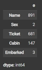
df[numeric_columns].nunique(): Returns count of unique values per column.
1
df[cat_col].nunique()
Output:
1
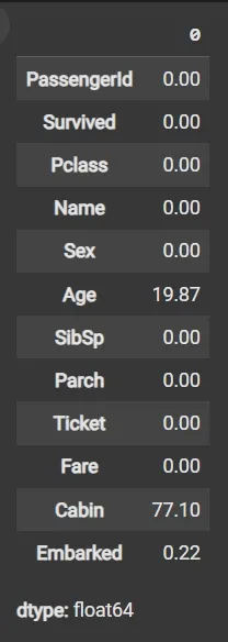
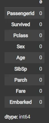
round((df.isnull().sum() / df.shape[0]) * 100, 2)
Output:
1
2
3
df1 = df.drop(columns=['Name', 'Ticket', 'Cabin'])
df1.dropna(subset=['Embarked'], inplace=True)
df1['Age'].fillna(df1['Age'].mean(), inplace=True)
1
2
3
4
5
6
7
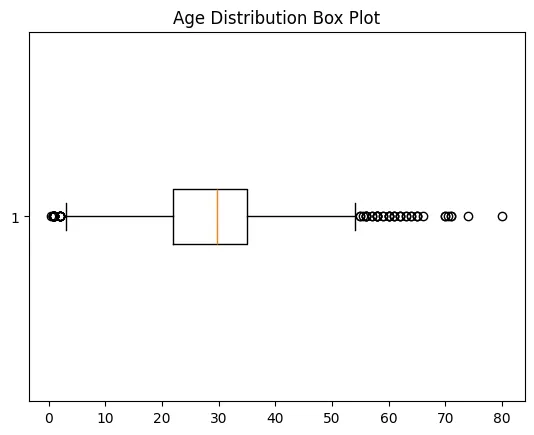
import matplotlib.pyplot as plt
plt.boxplot(df3['Age'], vert=False)
plt.ylabel('Variable')
plt.xlabel('Age')
plt.title('Box Plot')
plt.show()
Output:
1
2
3
4
5
6
7
mean = df1['Age'].mean()
std = df1['Age'].std()

lower_bound = mean - 2 * std
upper_bound = mean + 2 * std

df2 = df1[(df1['Age'] >= lower_bound) & (df1['Age'] <= upper_bound)]
1
2
df3 = df2.fillna(df2['Age'].mean())
df3.isnull().sum()
1
2
3
4
5
6
7
8
9
10
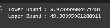
mean = df3['Age'].mean()
std = df3['Age'].std()
lower_bound = mean - 2 * std
upper_bound = mean + 2 * std
print('Lower Bound :', lower_bound)
print('Upper Bound :', upper_bound)
df4 = df3[(df3['Age'] >= lower_bound) & (df3['Age'] <= upper_bound)]
Output:
Data validation and verification involve ensuring that the data is accurate and consistent by comparing it with external sources or expert knowledge. For the machine learning prediction we separate independent and target features. Here we will consider only ‘Sex’ ‘Age’ ‘SibSp’, ‘Parch’ ‘Fare’ ‘Embarked’ only as the independent features and Survived as target variables because PassengerId will not affect the survival rate.
1
2
X = df3[['Pclass','Sex','Age', 'SibSp','Parch','Fare','Embarked']]
Y = df3['Survived']
Data formatting involves converting the data into a standard format or structure that can be easily processed by the algorithms or models used for analysis. Here we will discuss commonly used data formatting techniques i.e. Scaling and Normalization.
Scaling involves transforming the values of features to a specific range. It maintains the shape of the original distribution while changing the scale. It is useful when features have different scales and certain algorithms are sensitive to the magnitude of the features. Common scaling methods include:
1
2
3
4
5
6
7
8
from sklearn.preprocessing import MinMaxScaler
scaler = MinMaxScaler(feature_range=(0, 1))
num_col_ = [col for col in X.columns if X[col].dtype != 'object']
x1 = X
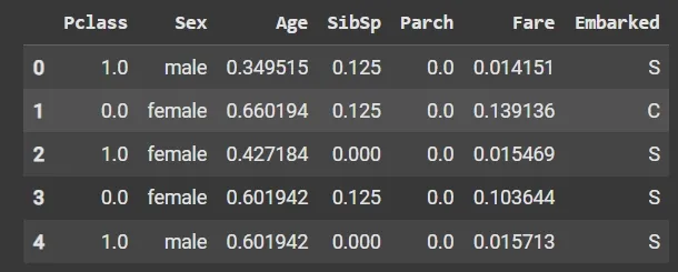
x1[num_col_] = scaler.fit_transform(x1[num_col_])
x1.head()
Output:
Standardization (Z-score scaling): Standardization transforms the values to have a mean of 0 and a standard deviation of 1. It centers the data around the mean and scales it based on the standard deviation. Standardization makes the data more suitable for algorithms that assume a Gaussian distribution or require features to have zero mean and unit variance.
\[Z = (X - μ) / σ\]Where:
- X = Data
- μ = Mean value of X
- σ = Standard deviation of X
Data normalization is a preprocessing method that resizes the range of feature values to a specific scale, usually between 0 and 1. It is a feature scaling technique used to transform data into a standard range. Normalization ensures that features with different scales or units contribute equally to the model and improves the performance of many machine learning algorithms.
Key Features of Normalization:
Machine learning models often assume that all features contribute equally. Features with different scales can dominate the model’s behavior if not scaled properly. Using normalization, we can:
Standardization, also called Z-score normalization is a separate technique. It transforms data so that it has a mean of 0 and a standard deviation of 1.
Standardization and Normalization are quite similar and confusing lets see the quick differences between them:
| Feature | Normalization (Min–Max) | Standardization (Z-score) |
|---|---|---|
| Goal | Rescale data to a specific range | Center data to mean 0, standard deviation 1 |
| Range of values | Fixed (e.g., 0–1) | Not fixed |
| Effect of outliers | Sensitive | Less sensitive |
| Assumes data distribution | No | Assumes roughly Gaussian |
| Use case | Distance-based algorithms | Algorithms assuming Gaussian or using regularization |
| Example | Scaling pixel values to [0,1] | Scaling test scores to z-scores |
Note: Normalization and Standardization are two distinct feature scaling techniques.
There are several techniques to normalize data, each transforming values to a common scale in different ways
Min-Max normalization rescales a feature to a specific range, typically [0, 1]:
\[X_{\text{normalized}} = \frac{X - X_{\min}}{X_{\max} - X_{\min}}\]
- The minimum value maps to 0
- The maximum value maps to 1
- Other values are scaled proportionally
Decimal scaling normalizes data by shifting the decimal point of values:
\[v' = \frac{v}{10^{j}}\]j is the smallest integer such that the maximum absolute value of v′ is less than 1
Log transformation compresses large values and spreads out small values:
\[X' = \log(X + 1)\]Scales a data vector to have a magnitude of 1:
\[X' = \frac{X}{\lVert X \rVert}\]
- Commonly used in text mining and machine learning algorithms like KNN
- Preserves direction but normalizes magnitude
We will import the necessary libraries like pandas and scikit-learn.
1
2
import pandas as pd
from sklearn.preprocessing import MinMaxScaler, StandardScaler
We will load the dataset and separate the features from the target variable.
1
2
3
4
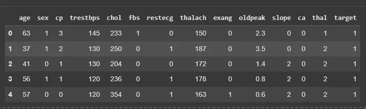
df = pd.read_csv('/content/heart.csv')
X = df.drop('target', axis=1)
y = df['target']
df.head()
Output:
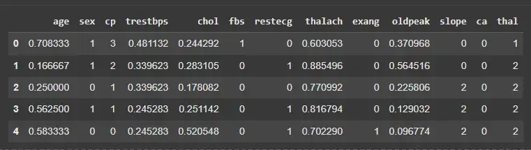
We will normalize selected numeric features to scale them between 0 and 1.
1
2
3
4
5
6
features = ['age','trestbps','chol','thalach','oldpeak']
scaler = MinMaxScaler()

X_normalized = X.copy()
X_normalized[features] = scaler.fit_transform(X[features])
X_normalized.head()
Output:
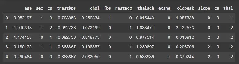
We will standardize the same features to have mean 0 and standard deviation 1.
Note: Standardization is less sensitive to outliers compared to normalization.
1
2
3
4
scaler_z = StandardScaler()
X_standardized = X.copy()
X_standardized[features] = scaler_z.fit_transform(X[features])
X_standardized.head()
Output: